Units and Constants

pysynphot understands some Flux Units and Wavelength Units that are commonly used in astronomy. Unit conversion can be easily done within spectral objects by using pysynphot.spectrum.SourceSpectrum.convert() (for flux and wavelength) and pysynphot.spectrum.SpectralElement.convert() (wavelength only, as throughput is unitless) methods. As in IRAF STSDAS SYNPHOT, only lowercase unit names are valid.

Unless explicitly stated otherwise in API documentations, all calculations are done in the following internal units first, and then presented in user-specified units:

Angstrom for wavelength
photlam for flux

Constants

These are the constants used in unit conversion:

Constant	Description	Value
`pysynphot.units.C`	Speed of light, c	\(2.99792458 \times 10^{18} \; \AA \; \mathrm{s}^{-1}\)
`pysynphot.units.H`	Planck’s constant, h	\(6.62620 \times 10^{-27} \; \mathrm{ergs} \; \mathrm{s}\)
`pysynphot.units.ABZERO`	`abmag` zero point	-48.6 mag
`pysynphot.units.STZERO`	`stmag` zero point	-21.1 mag

Flux Units

The recognized flux units for source spectrum and observation objects are as tabulated below. For IRAF STSDAS SYNPHOT users, the unit name is equivalent to form, which has become fluxunits in pysynphot (see Examples). Most calculation and sampling results are presented in the given flux unit (e.g., sample() and effstim()). Since all internal flux calculations are done using photlam, no special steps are necessary when an operation is done on source spectra with different flux units. Counts and Magnitudes further explains the units of vegamag, abmag, stmag, obmag, and counts. The rest of the supported flux units should be self-evident.

Name	Class Object	Unit
photlam	`Photlam`	\(\mathrm{photon} \; \mathrm{s}^{-1} \; \mathrm{cm}^{-2} \; \AA^{-1}\)
photnu	`Photnu`	\(\mathrm{photon} \; \mathrm{s}^{-1} \; \mathrm{cm}^{-2} \; \mathrm{Hz}^{-1}\)
flam	`Flam`	\(\mathrm{erg} \; \mathrm{s}^{-1} \; \mathrm{cm}^{-2} \; \AA^{-1}\)
fnu	`Fnu`	\(\mathrm{erg} \; \mathrm{s}^{-1} \mathrm{cm}^{-2} \mathrm{Hz}^{-1}\)
stmag	`STMag`	\(-2.5 \times \log(\mathrm{flam}) - 21.1\)
abmag	`ABMag`	\(-2.5 \times \log(\mathrm{fnu}) - 48.6\)
obmag	`OBMag`	\(-2.5 \times \log(\mathrm{count})\)
vegamag	`VegaMag`	\(-2.5 \times \log(\mathrm{flux} \; / \; \mathrm{flux}_{\mathrm{Vega}})\)
count counts	`Counts`	\(\mathrm{photon} \; \mathrm{s}^{-1}\)
jy	`Jy`	\(10^{-23} \; \mathrm{erg} \; \mathrm{s}^{-1} \; \mathrm{cm}^{-2} \mathrm{Hz}^{-1}\)
mjy	`mJy`	\(10^{-26} \; \mathrm{erg} \; \mathrm{s}^{-1} \; \mathrm{cm}^{-2} \mathrm{Hz}^{-1}\)
ujy mujy microjy	`muJy`	\(10^{-29} \; \mathrm{erg} \; \mathrm{s}^{-1} \; \mathrm{cm}^{-2} \mathrm{Hz}^{-1}\)
njy nanojy	`nJy`	\(10^{-32} \; \mathrm{erg} \; \mathrm{s}^{-1} \; \mathrm{cm}^{-2} \mathrm{Hz}^{-1}\)

Counts and Magnitudes

pysynphot supports counts and the following magnitude systems:

obmag, the instrumental magnitude that is the logarithmic form of counts. Conversion involving counts and obmag assumes a pre-defined telescope collecting area.
abmag, the \(\mathrm{AB}_{\nu}\) magnitude from Oke (1974), which is based on a constant flux density per unit frequency.
stmag, the \(\mathrm{ST}_{\lambda}\) or Space Telescope magnitude, which is based on a constant flux density per unit wavelength.
vegamag, which is defined by setting the magnitude of Vega to zero in all bands. The adopted Vega spectrum is defined over a wavelength range of 900 Angstroms to 300 microns.

vegamag offers a reasonable approximation to many of the conventional photometric systems that use the spectrum of Vega to define magnitude zero in one or more passbands. In broadband photometry, the relevant passband integral is calculated first for the source spectrum and then again for the spectrum of Vega, and the ratio of the two results is converted to a magnitude. This would not be a scientifically meaningful option for spectrophotometry.

Meanwhile, abmag and stmag are appropriate for either spectrophotometry or photometry. Their zero point values of 48.60 and 21.10 mag, respectively, are chosen for convenience so that Vega has \(\mathrm{AB}_{\nu}\) and \(\mathrm{ST}_{\lambda}\) magnitudes close to 0 in the Johnson V passband, as shown in the following figure:

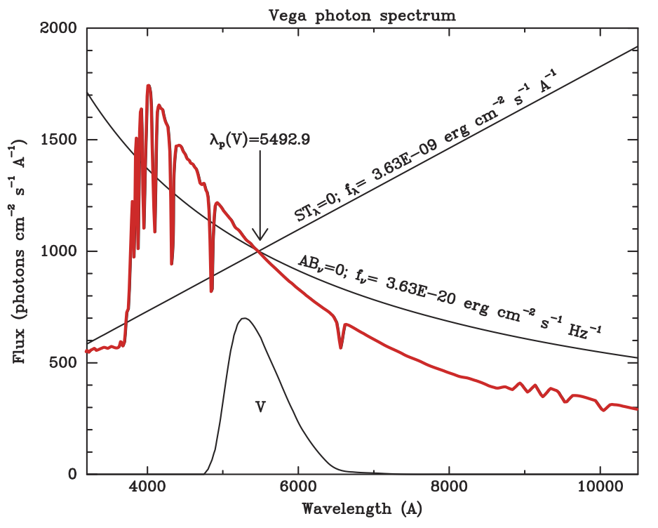
Standard photometric systems generally use the spectrum of Vega to define magnitude zero. The spectrophotometric magnitudes \(\mathrm{AB}_{\nu}\) and \(\mathrm{ST}_{\lambda}\) refer instead to spectra of constant \(f_{\nu}\) and \(f_{\lambda}\), respectively. Magnitude zero in both systems is defined to be the mean flux density of Vega in the Johnson V passband. Thus all three of the spectra shown here produce the same count rate in the Johnson V passband. The pivot wavelength of Johnson V is defined to be the crossing point of the \(\mathrm{AB}_{\nu}\)\(= 0\) and \(\mathrm{ST}_{\lambda}\)\(= 0\) spectra.

Because the abmag and stmag systems are defined such that they result in constant magnitudes for spectra having constant flux per unit frequency and wavelength, respectively, they will not provide magnitudes on a conventional system, such as UBVRI, without first deriving an appropriate transformation onto the desired standard system.

obmag and counts are used to predict detected count rates. For instance, countrate() calculates the predicted number of detected counts per second integrated over the passband. There are two important things to remember concerning this unit:

The number of counts per channel depends on the width (in wavelength space) of the channel in the wavelength grid that is used. As stated above, all flux calculations are done internally in the unit of photlam, so when the output unit of counts or obmag is requested, the photlam values are multiplied by the collecting area of the telescope and by the width (in Angstroms) of each channel in the wavelength grid. Therefore, in order to accurately predict the number of counts per channel for a spectroscopic instrument, it is necessary to use a wavelength grid that provides a good match to the dispersion properties of the selected instrument mode (see Wavelength Table). For supported HST instruments, the appropriate wavelength grid will be automatically selected.
The unit “counts” refers to the actual detector counts for the FOC, FOS, HRS, and HSP instruments. While for the WF/PC-1, WFPC2, NICMOS, WFC3, COS, ACS, and STIS instruments, it refers to electrons. In order to obtain counts in the unit of data number (DN) for some of the latter instruments, include the appropriate keyword for ADC gain, if supported (see Appendix B: OBSMODE Keywords).

Wavelength Units

These are the recognized wavelength units for all spectrum objects:

Name	Class Object	Unit
m meter	`Meter`	SI base unit for length
cm	`Cm`	\(10^{-2} \; \mathrm{m}\)
mm	`Mm`	\(10^{-3} \; \mathrm{m}\)
um micron microns	`Micron`	\(10^{-6} \; \mathrm{m}\)
nm	`Nm`	\(10^{-9} \; \mathrm{m}\)
angstrom angstroms	`Angstrom`	\(10^{-10} \; \mathrm{m}\)
1/um inversemicron inversemicrons	`InverseMicron`	\(10^{6} \; \mathrm{m}^{-1}\)
hertz	`Hz`	\(\mathrm{s}^{-1}\)

Examples

Create a source spectrum from arrays with default units:

>>> sp = S.ArraySpectrum(
...     np.array([1000, 2000, 3000]), np.array([0.1, 0.2, 0.3]))
>>> print('{0}, {1}'.format(sp.waveunits.name, sp.fluxunits.name))
angstrom, photlam

Convert both wavelength and flux units:

>>> sp.convert('nm')
>>> sp.convert('flam')
>>> print('{0}, {1}'.format(sp.waveunits.name, sp.fluxunits.name))
nm, flam
>>> sp.wave
array([ 100.,  200.,  300.])
>>> sp.flux
array([  1.98648479e-12,   1.98648479e-12,   1.98648479e-12])

To sample the spectrum in user units (i.e., nm and flam), use its sample() method:

>>> sp.sample(200)
1.9864847851996004e-12

To sample the spectrum in internal units (i.e., Angstrom and photlam), use its __call__() method:

>>> sp(2000)
0.20000000000000001