Tutorials

These tutorials are for those who prefer to jump right in. There are also some simple exercises for practice. You can skip the parts involving plotting if you do not have matplotlib installed.

Before starting the tutorials, see Installation and Setup.

Tutorial 1: The Basics

In this tutorial, you will be introduced to the pysynphot software and practice the following basic functionalities:

• Read spectra from files and display them using matplotlib

• Create analytic source spectra

• Create a bandpass from observation mode string expression

• Manipulate spectrum objects

• Create an observation and compute its count rate and effective wavelength

• Write out spectra as FITS tables

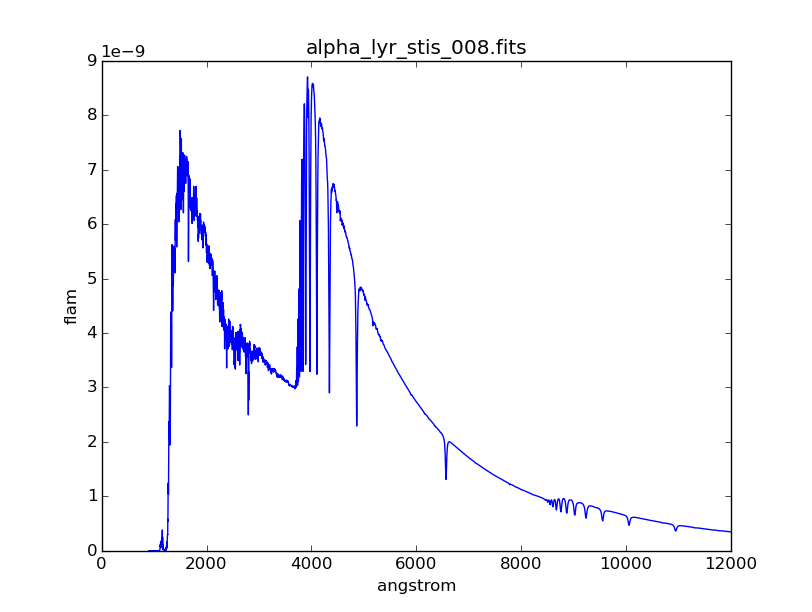
Source Spectrum from File

Read a Vega spectrum (not the built-in version) from FITS table and convert its flux unit to flam:

>>> vega_file = os.path.join(
...     os.environ['PYSYN_CDBS'], 'calspec', 'alpha_lyr_stis_005.fits')
>>> vega = S.FileSpectrum(vega_file)
>>> vega.convert('flam')

Evaluate flux at 5000 Angstroms:

>>> vega(5000)  # photlam (internal unit)
1190.0510381121621
>>> vega.sample(5000)  # flam (user unit)
4.7280365616415988e-09

Plot the Vega spectrum:

>>> plt.plot(vega.wave, vega.flux)
>>> plt.xlim(0, 12000)
>>> plt.xlabel(vega.waveunits)
>>> plt.ylabel(vega.fluxunits)
>>> plt.title(os.path.basename(vega.name))

Analytic Source Spectra

Create a blackbody source with a temperature of 40000 Kelvin:

>>> bb = S.BlackBody(40000)

Create a power-law source with reference wavelength of 10000 Angstrom and index of -2:

>>> plaw = S.PowerLaw(10000, -2)

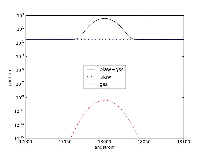
Create a Gaussian source with total flux of \(8.3 \times 10^{-9}\) flam under the curve, central wavelength of 18000 Angstroms, and FWHM of 20 Angstroms:

>>> gss = S.GaussianSource(8.3e-9, 18000, 20, fluxunits='flam')

Create a source that emits 1 count across all wavelengths:

>>> onecount = S.FlatSpectrum(1, fluxunits='counts')

Add Gaussian and power-law source spectra together to create a new source:

>>> sp = plaw + gss

Plot the combined spectrum and its individual components:

>>> plt.semilogy(sp.wave, sp.flux, 'k', label='plaw+gss')
>>> plt.semilogy(plaw.wave, plaw.flux, 'b:', label='plaw')
>>> plt.semilogy(gss.wave, gss.flux, 'r--', label='gss')
>>> plt.xlim(17900, 18100)
>>> plt.xlabel(sp.waveunits)
>>> plt.ylabel(sp.fluxunits)
>>> plt.legend(loc='center')

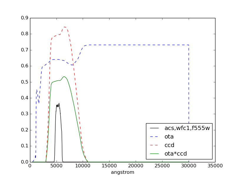
Bandpass from Observation Mode

Create a bandpass for HST/ACS instrument using its WFC1 detector and F555W filter:

>>> bp1 = S.ObsBandpass('acs,wfc1,f555w')

Show all the components in the light path used to create the bandpass:

>>> bp1.showfiles()
/my/local/dir/trds/comp/ota/hst_ota_007_syn.fits
/my/local/dir/trds/comp/acs/acs_wfc_im123_004_syn.fits
/my/local/dir/trds/comp/acs/acs_f555w_wfc_005_syn.fits
/my/local/dir/trds/comp/acs/acs_wfc_ebe_win12f_005_syn.fits
/my/local/dir/trds/comp/acs/acs_wfc_ccd1_mjd_021_syn.fits

Read the OTA and CCD transmissions from files, then multiply them:

>>> ota = S.FileBandpass('/my/local/dir/trds/comp/ota/hst_ota_007_syn.fits')
>>> ccd = S.FileBandpass(
...     '/my/local/dir/trds/comp/acs/acs_wfc_ccd1_mjd_021_syn.fits')
>>> bp2 = ota * ccd

Plot the bandpass and overlay its two components from above:

>>> plt.plot(bp1.wave, bp1.throughput, 'k', label='acs,wfc1,f555w')
>>> plt.plot(ota.wave, ota.throughput, 'b--', label='ota')
>>> plt.plot(ccd.wave, ccd.throughput, 'r--', label='ccd')
>>> plt.plot(bp2.wave, bp2.throughput, 'g', label='ota*ccd')
>>> plt.xlabel(bp1.waveunits)
>>> plt.legend(loc='best')

Spectrum Manipulation

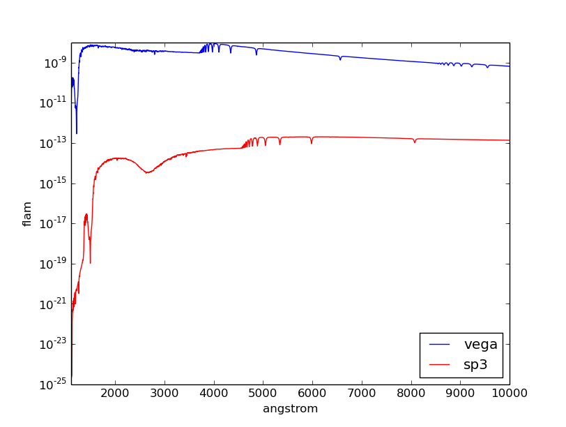
Get extinction curve for Milky Way (diffuse) with \(E(B-V) = 0.7\) and apply it to Vega spectrum from above. Then, check that the flux is indeed reduced by the extinction curve:

>>> extinct = S.Extinction(0.7, 'mwavg')
>>> extinct.citation
' Cardelli, Clayton, & Mathis (1989, ApJ, 345, 245) R_V = 3.10.'
>>> sp1 = vega * extinct
>>> max(vega.flux)
8.7730995298612719e-09
>>> max(sp1.flux)
5.06749522597244e-10

Redshift the reddened spectrum above by \(z = 0.23\). Then, check that the peak wavelength is indeed redder:

>>> sp2 = sp1.redshift(0.23)  # sp2 is in PHOTLAM
>>> sp2.convert('flam')
>>> sp1.wave[sp1.flux == max(sp1.flux)][0]
5026.7534
>>> sp2.wave[sp2.flux == max(sp2.flux)][0]
6182.9067

Normalize the redshifted spectrum to a total flux of \(1.8 \times 10^{-13}\) flam over HST/ACS WFC1 F555W bandpass from above:

>>> sp3 = sp2.renorm(1.8e-13, 'flam', bp1)

Plot the resultant spectrum and compare to the original Vega:

>>> plt.semilogy(vega.wave, vega.flux, 'b', label='vega')
>>> plt.semilogy(sp3.wave, sp3.flux, 'r', label='sp3')
>>> plt.xlim(1100, 10000)
>>> plt.xlabel(vega.waveunits)
>>> plt.ylabel(vega.fluxunits)
>>> plt.legend(loc='lower right')

Observation

Create an observation using modified Vega spectrum and HST/ACS WFC1 F555W bandpass from above:

>>> obs = S.Observation(sp3, bp1)

Calculate count rate of this observation in the unit of counts/s over the HST collecting area (i.e., the primary mirror) that is defined in \(\mathrm{cm}^{2}\):

>>> obs.primary_area
45238.93416
>>> obs.countrate()
909477.56364769232

Calculate the count rate in \(\mathrm{counts} \; \mathrm{s}^{-1} \; \mathrm{cm}^{-2}\):

>>> obs.countrate() / obs.primary_area
20.103868062653145

Calculate the effective stimulus in flam:

>>> obs.effstim('flam')
1.7999999531057673e-13

Calculate effective wavelength in Angstroms:

>>> obs.efflam()
5425.0867727745972

Convert the flux unit to counts:

>>> obs.convert('counts')

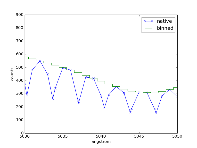
Plot observation data in both native and binned wavelength sets. Note that counts per wavelength bin depends on the size of the bin because it is not a flux density:

>>> plt.plot(obs.wave, obs.flux, marker='x', label='native')
>>> plt.plot(obs.binwave, obs.binflux, drawstyle='steps-mid', label='binned')
>>> plt.xlim(5030, 5050)
>>> plt.xlabel(obs.waveunits)
>>> plt.ylabel(obs.fluxunits)
>>> plt.legend(loc='best')

Write the observation out to two FITS tables, one with native dataset and the other binned:

>>> obs.writefits('myobs_native.fits', binned=False)
>>> obs.writefits('myobs_binned.fits')

Tutorial 2: Adding Emission Line

This tutorial is adapted from Exposure Time Calculator User’s Guide on a similar topic. In this tutorial, you will learn how to manipulate and superimpose an emission line to a continuum spectrum.

Create a continuum spectrum of a 5500 K blackbody with \(z = 0.6\):

>>> bb = S.BlackBody(5500).redshift(0.6)

Create a Gaussian emission line with \(8 \times 10^{-14}\) flam total flux under the curve and FWHM of 100 Angstroms centered at 7000 Angstroms:

>>> em = S.GaussianSource(8e-14, 7000, 100, fluxunits='flam')

Add emission line to continuum spectrum:

>>> sp = bb + em

Apply extinction curve for LMC (average) with \(E(B-V) = 1.3\) to the composite spectrum:

>>> my_spec = sp * S.Extinction(1.3, 'lmcavg')

Plot the result:

>>> plt.plot(my_spec.wave, my_spec.flux)
>>> plt.xlabel(my_spec.waveunits)
>>> plt.ylabel(my_spec.fluxunits)

Tutorial 3: FWHM

This tutorial is adapted from an example in the documentation of IRAF STSDAS SYNPHOT bandpar task. In this tutorial, you will learn how to calculate the full-width at half-maximum (FWHM) of the HST/WFPC instrument with F555W filter.

Create the bandpass:

>>> bp = S.ObsBandpass('wfpc,f555w')

Compute FWHM in Angstroms:

>>> np.sqrt(8 * np.log(2)) * bp.photbw()
1200.923243227332

Tutorial 4: Color Difference

This tutorial is adapted from an example in the documentation of IRAF STSDAS SYNPHOT calcphot task. In this tutorial, you will learn how to find the color difference of a 2500 K blackbody in Cousins I and HST/WFC3 UVIS1 F814W bandpasses.

Create the blackbody:

>>> bb = S.BlackBody(2500)

Create an observation for each of the two bandpasses. Cousins I bandpass does not have pre-defined binset, so for consistency with the other bandpass, it is to use the binning of HST/WFC3 UVIS1 detector:

>>> obs_wfc3 = S.Observation(bb, S.ObsBandpass('wfc3,uvis1,f814w'))
>>> obs_i = S.Observation(bb, S.ObsBandpass('i'), binset=obs_wfc3.binwave)

The color difference in magnitude is computed by subtracting the effective stimuli of the two observations. In instrumental magnitude, this is:

>>> obs_i.effstim('obmag') - obs_wfc3.effstim('obmag')
-1.2585631331417577

The color difference in linear flux unit is computed by dividing the effective stimuli of the two observations. In flam, this is:

>>> obs_i.effstim('flam') / obs_wfc3.effstim('flam')
0.95505705250139461

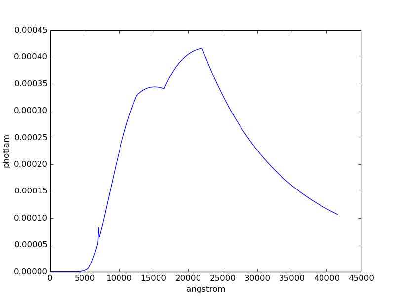
Tutorial 5: Continuum-Normalized Spectrum

In this tutorial, you will learn how to create a composite spectrum with a noisy blackbody continuum, an emission line, and an absorption line. Then, you will divide it by a smooth continuum and plot the resultant continuum-normalized spectrum.

Create the smooth continuum that is a 5000 K blackbody:

>>> bb = S.BlackBody(5000)

Add random noise to the continuum. Since pysynphot object cannot be multiplied with Numpy array, this has to be done indirectly by applying the noise to sampled flux array, and then use the results to build a new source spectrum:

>>> w = bb.wave
>>> nse = 1 + np.random.normal(size=w.size, scale=0.02)
>>> bb_noisy = S.ArraySpectrum(wave=w, flux=bb(w)*nse)

Apply emission and absorption lines to the noisy continuum. How to construct a Gaussian source is explained in Tutorial 1: Analytic Source Spectra:

>>> g_em = S.GaussianSource(0.02, 15000, 500, fluxunits='photlam')
>>> g_ab = S.GaussianSource(0.015, 4500, 100, fluxunits='photlam')
>>> sp = bb_noisy + g_em - g_ab

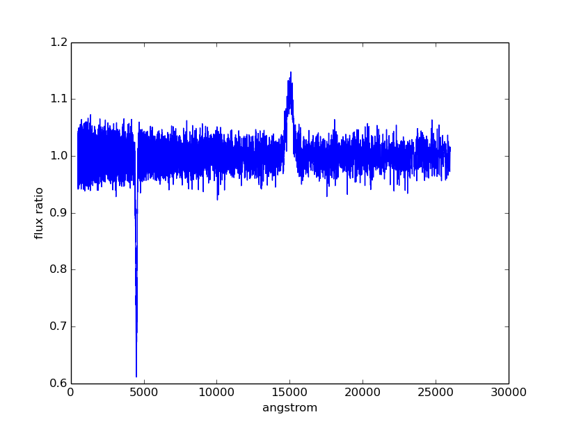
Divide the spectrum above with the smooth continuum to obtain flux ratio. Since pysynphot object cannot do division, this has to be calculated indirectly using sampled flux arrays, which happen to be in photlam in this example:

>>> fratio = sp(w) / bb(w)

Plot the continuum-normalized spectrum:

>>> plt.plot(w, fratio)
>>> plt.xlabel(sp.waveunits)
>>> plt.ylabel('flux ratio')

Tutorial 6: Custom Wavelength Table

In this tutorial, you will learn how to create a custom wavelength array and save it to a FITS table using astropy.io.fits. Then, you will read the array back in from file, and use it to define binned dataset in an observation.

Suppose we want a wavelength set that ranges from 2000 to 8000 Angstroms, with 1 Angstrom spacing over most of the range, but 0.1 Angstrom spacing around the [O III] forbidden lines at 4959 and 5007 Angstroms.

Create the 3 regions separately, concatenate them, and display the result:

>>> lowwave = np.arange(2000, 4950)
>>> midrange = np.arange(4950, 5010, 0.1)  # [O III]
>>> hiwave = np.arange(5010, 8000)
>>> wave = np.concatenate([lowwave, midrange, hiwave])
>>> wave
array([ 2000.,  2001.,  2002., ...,  7997.,  7998.,  7999.], dtype=float32)

Create a FITS table column from the concatenated array above, insert it into a new FITS table, and write the table out to file:

>>> from astropy.io import fits
>>> col = fits.Column(
...     name='wavelength', unit='angstroms', format='E', array=wave)
>>> tabhdu = fits.BinTableHDU.from_columns([col])
>>> tabhdu.writeto('mywaveset.fits', clobber=True)

Read the custom wavelength set back in from file:

>>> with fits.open('mywaveset.fits') as pf:
...     wave = pf[1].data.field('wavelength')

Create an observation of Vega with HST/ACS WFC1 F555W bandpass, using the custom wavelength set for binned data, and then check that the binned wavelength set is indeed the given one:

>>> obs = S.Observation(S.Vega, S.ObsBandpass('acs,wfc1,f555w'), binset=wave)
>>> obs.binwave
array([ 2000.,  2001.,  2002., ...,  7997.,  7998.,  7999.], dtype=float32)

Tutorial 7: Count Rates for Multiple Apertures

In this tutorial, you will learn how to calculate count rates for observations of the same source and bandpass, but with different apertures. Note that this feature is only available for observing modes that allow encircled energy (EE) radius specification (see Appendix B: OBSMODE Keywords).

Create two observations of Vega (renormalized to 20 stmag in Johnson V) with HST/ACS WFC1 F555W bandpass, with 0.3 and 1.0 arcsec EE radii, respectively:

>>> sp = S.Vega.renorm(20, 'stmag', S.ObsBandpass('johnson,v'))
>>> obs03 = S.Observation(sp, S.ObsBandpass('acs,wfc1,f555w,aper#0.3'))
>>> obs10 = S.Observation(sp, S.ObsBandpass('acs,wfc1,f555w,aper#1.0'))

Calculate the count rates for both and display the results:

>>> c03 = obs03.countrate()
>>> c10 = obs10.countrate()
>>> print('Count rate for 0.3" is {0}\n'
...       'Count rate for 1.0" is {1}'.format(c03, c10))
Count rate for 0.3" is 174.063405183
Count rate for 1.0" is 185.733901828

Tutorial 8: Blueshift

In this tutorial, you will learn how to blueshift an observed spectrum back to its rest frame. The blueshift value, \(z_{\mathrm{blue}}\), can be calculated from the redshift, \(z\), as follows:

\[z_{\mathrm{blue}} = \frac{1}{1 + z} - 1\]

Create an observed blackbody spectrum at \(z = 0.1\) (this is similar to the example in Redshift):

>>> z = 0.1
>>> bb = S.BlackBody(5000)
>>> sp_obs = bb.redshift(z)

Calculate and apply the blueshift, and then compare the result to the expected values at rest frame (i.e., the original blackbody spectrum):

>>> z_blue = 1.0 / (1 + z) - 1
>>> sp_rest = sp_obs.redshift(z_blue)
>>> np.testing.assert_allclose(sp_rest.wave, bb.wave)
>>> np.testing.assert_allclose(sp_rest.flux, bb.flux)

Tutorial 9: Bandpass stmag Zeropoint

HST bandpasses store their Bandpass Unit Response values under the PHOTFLAM keyword in image headers. This keyword is then used to compute stmag zeropoint for the respective bandpass (e.g., ACS and WFC3).

In this tutorial, you will learn how to calculate the stmag zeropoint for the F555W filter in HST/ACS WFC1 detector:

>>> bp = S.ObsBandpass('acs,wfc1,f555w')
>>> st_zpt = -2.5 * np.log10(bp.unit_response()) - 21.1
>>> print('STmag zeropoint for {0} is {1:.5f}'.format(bp.name, st_zpt))
STmag zeropoint for acs,wfc1,f555w is 25.65880

Tutorial 10: Spectrum from Custom Text File

In this tutorial, you will learn how to load a source spectrum from an ASCII table that does not conform to the expected format stated in File I/O. Since FileSourceSpectrum does not allow explicit setting of units, if your table data have non-default wavelength or flux units, you have to first load them into Numpy arrays and then use ArraySourceSpectrum to obtain the spectrum object correctly. Similar workflow applies to bandpass for non-default wavelength units, using ArraySpectralElement (not shown).

Let’s say your ASCII table looks like this:

# My source spectrum
# ROW    WAVELENGTH(NM)    FLUX(PHOTLAM)
1        400.0             0.1
2        401.0             0.1234
3        405.0             0.4556
...      ...               ...

There are many ways you can read the ASCII table into Numpy arrays. The example below uses Astropy:

>>> from astropy.io import ascii
>>> tab = ascii.read('myfile.txt', names=['row', 'wave', 'flux'])
>>> wave = tab['wave']  # Second column
>>> flux = tab['flux']  # Third column

Construct the source spectrum from the arrays above:

>>> sp = S.ArraySpectrum(
...     wave=wave, flux=flux, waveunits='nm', fluxunits='photlam')

Exercises

Here are the exercises for those who wish to apply what they learned from some of the tutorials above. Answers are not provided, but should be obvious based on the available tutorials and documentation.

Tutorial 1: The Basics

1. Convert the blackbody source created in Tutorial 1 to flam flux unit. Plot it.

2. Create a bandpass for HST/WFC3 instrument using its UVIS1 detector and F475W filter. Plot it.

3. Create an observation using the blackbody source and the HST/WFC3 UVIS1 F475W bandpass. Compute its count rate. Plot it.

Tutorial 2: Adding Emission Line

1. Create a Gaussian emission line with \(10^{-13}\) flam total flux under the curve and FWHM of 50 Angstroms centered at 5000 Angstroms. Redshift it by \(z=0.01\).

2. Add this new emission line to the composite spectrum from Tutorial 2. Don’t forget to account for the foreground LMC extinction.

3. Plot your result. You should see the same composite spectrum as in the tutorial but with an extra emission line that you created.

Tutorial 3: FWHM

1. Find the FWHM for HST/ACS WFC1 F555W bandpass.

2. Find the FWHM for a box-shaped bandpass centered at 3500 Angstroms with the width of 100 Angstroms.

Tutorial 4: Color Difference

1. Find the color difference for the observations in Tutorial 4 in stmag.

2. Find the color difference for the observations in Tutorial 4 in counts/s.

Tutorial 5: Continuum-Normalized Spectrum

1. Repeat the steps in Tutorial 5 but using blackbody temperature of 10000 Kelvin.

2. Add a new absorption line of your choice to the spectrum that you just created. Recalculate and replot its flux ratio.