Switching from IRAF STSDAS SYNPHOT

This section provides basic switcher’s guide for those who are familiar with IRAF STSDAS SYNPHOT. This guide is not meant to be all-inclusive for two reasons:

• Some of the SYNPHOT tasks can be reproduced in several different ways using pysynphot.

• Not all the SYNPHOT tasks are available in pysynphot.

The agreement of results between these two software were discussed in detail in TSR 2009-01: Pysynphot Commissioning Report (Laidler 2009).

In the tables below:

• sp represents a source spectrum

• bp represents a bandpass

• obs represents an observation

Source Spectrum

pysynphot	SYNPHOT
S.FileSpectrum(filename)	spec(filename)
S.BlackBody(temperature)	bb(temperature)
S.FlatSpectrum(val, fluxunits=form)	unit(val, form)
S.Powerlaw(refval, expon, fluxunits=form)	pl(refval, expon, form)
S.GaussianSource(totflux, mu, fwhm, fluxunits=form)	em(mu, fwhm, totflux, form)
S.ArraySpectrum(wave, flux, fluxunits=form)	N/A
S.Icat(model, Teff, Z, log_g)	icat(model, Teff, Z, log_g)
sp.renorm(val, form, bp)	rn(sp, bp, val, form)
sp.redshift(z)	z(sp, z)
sp.writefits(filename)	calcspec sp filename
plt.plot(sp.wave, sp.flux)	N/A

Bandpass

There is no single bandpass method that is equivalent to IRAF STSDAS SYNPHOT bandpar task, but different commands can be used separately in order to derive different photometric properties, as tabulated below.

pysynphot	SYNPHOT
S.FileBandpass(filename)	thru(filename)
S.Box(mu, width)	box(mu, width)
S.ObsBandpass(obsmode)	band(obsmode)
bp.avgwave()	bandpar bp photlist=avglam
bp.efficiency()	bandpar bp photlist=qtlam
bp.equivwidth()	bandpar bp photlist=equvw
bp.rectwidth()	bandpar bp photlist=rectw
bp.photbw()	bandpar bp photlist=bandw
bp.throughput.max()	bandpar bp photlist=tpeak
bp.thermback()	thermback obsmode
bp.writefits(filename)	calcband bp filename
plt.plot(bp.wave, bp.throughput)	plband bp

Observation

pysynphot	SYNPHOT
S.Observation(sp, bp)	N/A
obs.countrate()	calcphot bp sp counts
obs.effstim(form)	calcphot bp sp form
obs.efflam()	calcphot bp sp flam func=’efflerg’
obs.writefits(filename)	N/A
plt.plot(obs.binwave, obs.binflux)	plspec bp sp photlam

Miscellaneous

pysynphot	SYNPHOT
S.Extinction(val, law)	ebmvx(val, law)
S.Extinction(val, ‘gal1’)	ebmv(val)
S.Waveset(w1, w2, dw)	genwave filename w1 w2 dw

Language Parser

pysynphot also has a special parser that can read some of the legacy SYNPHOT language for spectrum objects. However, the parser cannot perform legacy commands such as calcphot or bandpar.

The following table lists the available operations:

Parser Syntax	Pythonic Equivalent
band(obsmode)	S.ObsBandpass(obsmode)
bb(temperature)	S.BlackBody(temperature)
box(mu, width)	S.Box(mu, width)
ebmvx(val, law)	S.Extinction(val, law)
em(mu, fwhm, totflux, form)	S.GaussianSource(totflux, mu, fwhm, fluxunits=form)
icat(model, Teff, Z, log_g)	S.Icat(model, Teff, Z, log_g)
pl(refval, expon, form)	S.Powerlaw(refval, expon, fluxunits=form)
rn(sp, bp, val, form)	sp.renorm(val, form, bp)
spec(filename)	S.FileSpectrum(filename)
unit(val, form)	S.FlatSpectrum(val, fluxunits=form)
z(sp, z)	sp.redshift(z)

These are the flux units (form) recognized by the parser (for wavelength, only Angstrom is accepted):

• fnu

• flam

• photnu

• photlam

• counts

• abmag

• stmag

• obmag

• vegamag

• jy

• mjy

These are the reddening laws recognized by the parser. They are used for the law variable in the ebmvx command above:

• gal1

• gal3

• smc

• lmc

• xgal

This example shows how a blackbody can be generated using the parser and the regular Python class. It also shows that they are both the same thing:

>>> from pysynphot import spparser as P
>>> bb1 = P.parse_spec('bb(5000)')
>>> bb2 = S.BlackBody(5000)   # Equivalent to bb1
>>> assert bb1.integrate() == bb2.integrate()

Meanwhile, this example shows how to use the parser to apply extinction to a redshifted and renormalized spectrum obtained from a catalog. It also generates the same spectrum using regular Python commands, and compares them:

>>> sp1 = P.parse_spec('ebmvx(0.1, lmc) * z(rn(icat(k93models, 5000, -0.5, 4.4), band(johnson,v), 18, abmag), 0.01)')
>>> sp2 = S.Extinction(0.1, 'lmc') * S.Icat('k93models', 5000, -0.5, 4.4).renorm(18, 'abmag', S.ObsBandpass('johnson,v')).redshift(0.01)
>>> assert sp1.integrate() == sp2.integrate()

Examples

In the examples below, the SYNPHOT commands are preceded by sy>. They are followed by the pysynphot equivalent in >>>. Some examples are adapted from SYNPHOT documentation.

IRAF STSDAS SYNPHOT setup:

iraf> stsdas
iraf> hst_calib
iraf> synphot
sy>

Calculate the pivot wavelength and the total flux (in counts/s) of a 5000 K blackbody in the HST/WFPC F555W bandpass. The blackbody spectrum is normalized to have a V magnitude of 18.6:

sy> calcphot "band(wfpc,f555w)" "rn(bb(5000),band(v),18.6,vegamag)" counts
Mode = band(wfpc,f555w)
Pivot       Equiv Gaussian
Wavelength  FWHM
5467.653    1200.953    band(wfpc,f555w)
Spectrum:  rn(bb(5000),band(v),18.6,vegamag)
VZERO      (COUNTS s^-1 hstarea^-1)
0.           419.5938

>>> obs = S.Observation(
...     S.BlackBody(5000).renorm(18.6, 'vegamag', S.ObsBandpass('v')),
...     S.ObsBandpass('band(wfpc,f555w)'))
>>> obs.bandpass.pivot()
5467.6512917540995
>>> obs.countrate()
418.74429418688777

Calculate the total flux (in obmag) of a 5000 K blackbody in the HST/ACS WFC1 F555W bandpass for \(E(B-V)\) values of 0.0, 0.25, and 0.5:

sy> calcphot "acs,wfc1,f555w" "bb(5000)*ebmv($0)" obmag vzero="0.0,0.25,0.5"
Mode = band(acs,wfc1,f555w)
Pivot       Equiv Gaussian
Wavelength  FWHM
5361.008    847.9977    band(acs,wfc1,f555w)
Spectrum:  bb(5000)*ebmv($0)
VZERO      (OBMAG s^-1 hstarea^-1)
0.           -10.0087
0.25         -9.1981
0.5          -8.39187

>>> for ebv in (0.0, 0.25, 0.5):
...     obs = S.Observation(
...         S.BlackBody(5000) * S.Extinction(ebv, 'gal1'),
...         S.ObsBandpass('acs,wfc1,f555w'))
...     print('{0}\t{1:.4f}'.format(ebv, obs.effstim('obmag')))
0.0     -10.0087
0.25    -9.1981
0.5     -8.3919

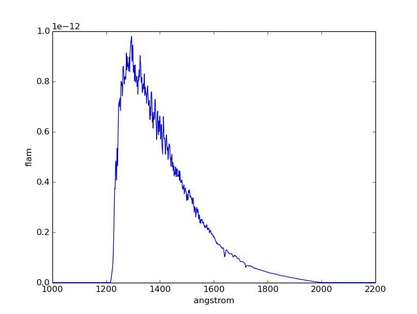
Plot an observation of BD+75 325 using the HST/ACS SBC F125LP bandpass in the unit of flam. The spectral data for BD+75 325 are stored in $PYSYN_CDBS/calspec/bd_75d325_stis_003.fits file. Because this spectrum has been arbitrarily normalized in intensity, we must first renormalize it to its proper U magnitude of 9.5:

sy> plspec "acs,sbc,f125lp" "rn(crcalspec$bd_75d325_stis_003.fits,band(u),9.5,vegamag)" flam

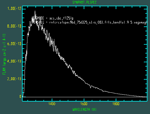
>>> filename = os.path.join(
...     os.environ['PYSYN_CDBS'], 'calspec', 'bd_75d325_stis_003.fits')
>>> obs = S.Observation(
...     S.FileSpectrum(filename).renorm(9.5, 'vegamag', S.ObsBandpass('u')),
...     S.ObsBandpass('acs,sbc,f125lp'))
>>> obs.convert('flam')
>>> plt.plot(obs.wave, obs.flux)
>>> plt.xlim(1000, 2200)
>>> plt.xlabel(obs.waveunits)
>>> plt.ylabel(obs.fluxunits)