Source Spectrum

A source spectrum is used to represent astronomical sources, such as stars and galaxies. It can be constructed in several different ways. An observation is a special case of a source spectrum that is convolved with a bandpass.

A source spectrum has these main components:

• flux

• fluxunits (see Flux Units)

• isAnalytic (This is True if the spectrum can be defined by a mathematical formula. For instance, a Gaussian spectrum is analytic, but an empirical spectrum is not.)

• name (Description of the spectrum; Also accessible via __str__())

• wave (a.k.a. waveset)

• waveunits (see Wavelength Units)

To evaluate its flux at a given wavelength, use its sample() (uses fluxunits) or __call__() (uses photlam) method, as given in the following example. Internally, evaluation uses numpy.interp().

>>> sp = S.Vega
>>> sp.fluxunits.name
'flam'
>>> sp.sample(5000)  # flam
4.7280365616415988e-09
>>> sp(5000)  # photlam
1190.0510381121621

Creating a Source

A source spectrum can be constructed by one of the following methods:

• Using a pre-defined function (Blackbody Radiation, Gaussian Emission, Power-Law, or Flat)

• Using built-in Vega spectrum

• Reading from spectral atlas or catalog

• Loading from a FITS or ASCII table

• Using your own wavelength and flux arrays

• Thermal spectrum is available for IR instruments but is usually not used directly

Blackbody Radiation

Blackbody radiation is defined by Planck’s law (Rybicki & Lightman 1979):

\[B_{\lambda}(T) = \frac{2 h c^{2} / \lambda^{5}}{\exp(h c / \lambda k T) - 1}\]

where the unit of \(B_{\lambda}(T)\) is flam per steradian.

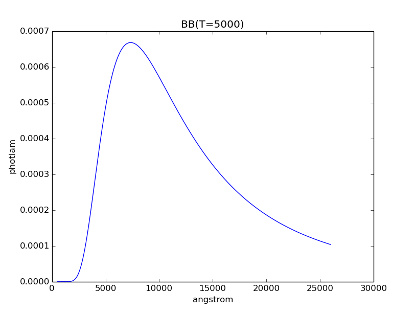
BlackBody generates a blackbody spectrum in photlam for a given temperature, normalized to a star of \(1 R_{\odot}\) at a distance of 1 kpc. Its waveset is taken from Reference Data.

The example below creates a blackbody spectrum at 5000 Kelvin:

>>> bb = S.BlackBody(5000)
>>> plt.plot(bb.wave, bb.flux)
>>> plt.xlabel(bb.waveunits)
>>> plt.ylabel(bb.fluxunits)
>>> plt.title(bb.name)

Gaussian Emission

GaussianSource could be used to represent an emission line:

\[ \begin{align}\begin{aligned}\sigma = \frac{\mathrm{FWHM}}{2 \; \sqrt{2 \; ln \; 2}}\\A = \frac{f_{\mathrm{tot}}}{\sqrt{2 \pi} \; \sigma}\\\mathrm{flux} = A \; / \; \exp(\frac{(x - x_{0})^{2}}{2 \; \sigma^{2}})\end{aligned}\end{align} \]

where

• FWHM is the full-width at half-maximum

• \(x_{0}\) is the central wavelength

• \(x\) is the wavelength array

• \(A\) is the amplitude at \(x_{0}\)

• \(f_{\mathrm{tot}}\) is the total flux under the curve

Its waveset is defined such that the spectrum is more tightly sampled around the peak. To create an absorption line, instead of adding the Gaussian source to the continuum spectrum, you subtract it.

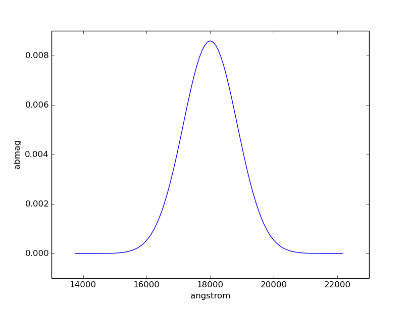
The example below creates a Gaussian source spectrum with total flux of 18.3 abmag under the curve, central wavelength of 18000 Angstroms, and FWHM of 2000 Angstroms:

>>> gs = S.GaussianSource(18.3, 18000, 2000, fluxunits='abmag')
>>> gs.name
'Gaussian: mu=18000 angstrom,fwhm=2000 angstrom, total flux=18.3 abmag'
>>> plt.plot(gs.wave, gs.flux)
>>> plt.xlabel(gs.waveunits)
>>> plt.ylabel(gs.fluxunits)

Power-Law

Powerlaw (also callable as pysynphot.PowerLaw) generates a power-law source:

\[\mathrm{flux} = (x \; / \; x_{0})^{-\alpha}\]

where

• \(x_{0}\) is the reference wavelength

• \(x\) is the wavelength array

• \(\alpha\) is the powerlaw index

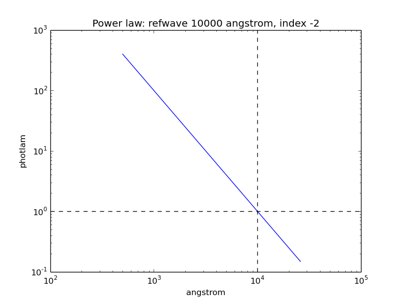
It is defined such that the flux is 1 (in given flux unit) at the reference wavelength. Its waveset is taken from Reference Data.

The example below creates a power-law source spectrum with reference wavelength of 10000 Angstroms and index of -2:

>>> pl = S.PowerLaw(10000, -2)
>>> plt.loglog(pl.wave, pl.flux)
>>> plt.axvline(10000, ls='--', color='k')
>>> plt.axhline(1, ls='--', color='k')
>>> plt.xlabel(pl.waveunits)
>>> plt.ylabel(pl.fluxunits)
>>> plt.title(pl.name)

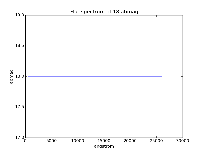
Flat

FlatSpectrum generates a flat spectrum that has a constant flux value in the given unit. Note that flux that is constant in a given unit might not be constant in another, as illustrated in the example below. Its waveset is taken from Reference Data.

The example below creates a source spectrum that is flat in abmag with the amplitude of 18 mag:

>>> flatsp = S.FlatSpectrum(18, fluxunits='abmag')
>>> plt.plot(flatsp.wave, flatsp.flux)
>>> plt.xlabel(flatsp.waveunits)
>>> plt.ylabel(flatsp.fluxunits)
>>> plt.title(flatsp.name)

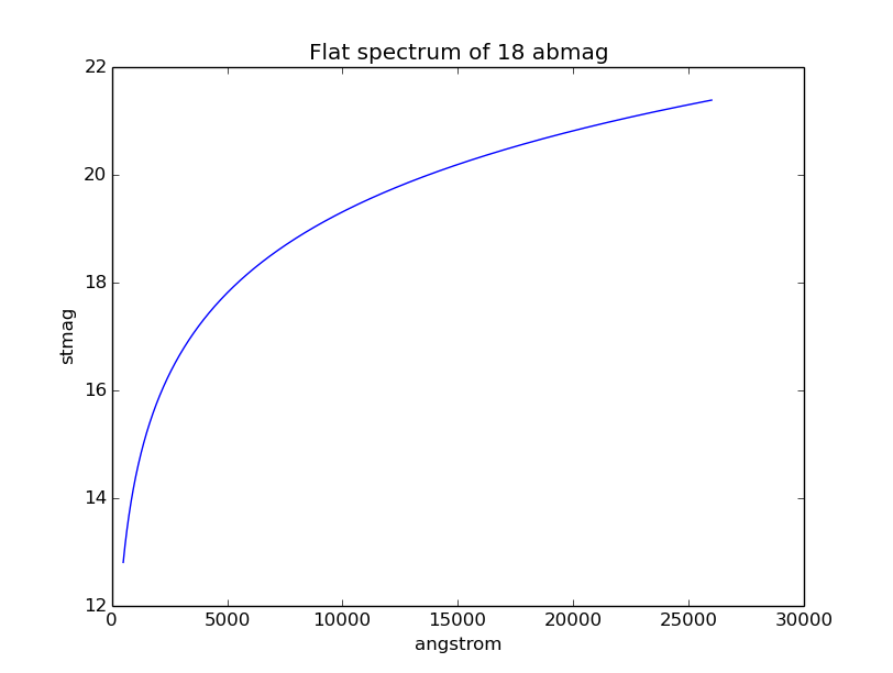
The spectrum above, however, is not flat in stmag:

>>> flatsp.convert('stmag')
>>> plt.plot(flatsp.wave, flatsp.flux)
>>> plt.xlabel(flatsp.waveunits)
>>> plt.ylabel(flatsp.fluxunits)
>>> plt.title(flatsp.name)

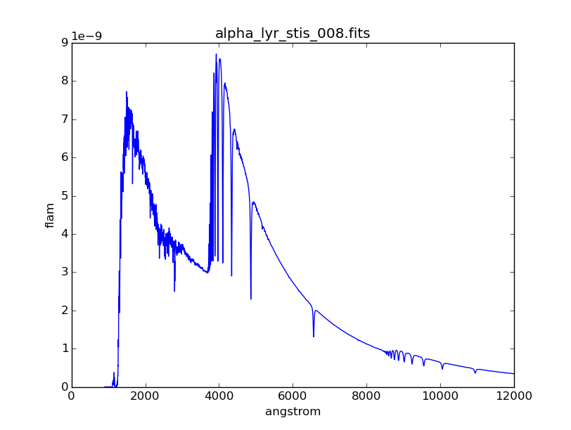
Vega

pysynphot uses built-in Vega spectrum for vegamag calculations. This spectrum comes with the package and is defined by pysynphot.locations.VegaFile, which is loaded on import as pysynphot.spectrum.Vega (also callable as pysynphot.Vega). Other versions of Vega spectrum are available as $PYSYN_CDBS/calspec/alpha_lyr_*.fits, which can be read using File I/O (also see HST Calibration Spectra).

The example below shows the built-in Vega spectrum:

>>> plt.plot(S.Vega.wave, S.Vega.flux)
>>> plt.xlim(0, 12000)
>>> plt.xlabel(S.Vega.waveunits)
>>> plt.ylabel(S.Vega.fluxunits)
>>> plt.title(os.path.basename(S.Vega.name))

Catalogs and Spectral Atlases

There are many spectral atlases consisting of both observed and model data that are available for use with pysynphot.

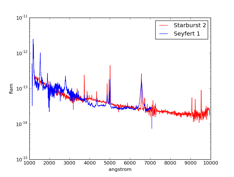
Plotting the spectra is a handy way to explore the contents. For instance, you are interested in making some HST observations of Seyfert galaxies and want to see what sort of template spectra are available to be used with pysynphot to predict observed count rates. In this case, a good place to look would be in AGN Atlas or Kinney-Calzetti Atlas. The example below plots the spectra of a starburst and a Seyfert 1 galaxies from their respective atlases:

>>> starburst = S.FileSpectrum(os.path.join(
...     os.environ['PYSYN_CDBS'], 'grid', 'kc96', 'starb2_template.fits'))
>>> seyfert1 = S.FileSpectrum(os.path.join(
...     os.environ['PYSYN_CDBS'], 'grid', 'agn', 'seyfert1_template.fits'))
>>> plt.semilogy(starburst.wave, starburst.flux, 'r', label='Starburst 2')
>>> plt.semilogy(seyfert1.wave, seyfert1.flux, 'b', label='Seyfert 1')
>>> plt.xlabel(starburst.waveunits)
>>> plt.ylabel(starburst.fluxunits)
>>> plt.legend()

For most of the catalogs and atlases (except the three mentioned below), you can load a spectrum from file once you have identified the desired filename that corresponds to the spectral parameters that you want, as shown in the example above.

However, three of the atlases (Castelli-Kurucz Atlas, Kurucz Atlas, and Phoenix Models) have a grid of basis spectra which are indexed for various combinations of effective temperature (\(T_{\mathrm{eff}}\)) in Kelvin, metallicity ([M/H]), and log surface gravity (\(\log g\)). They are best accessed with a special Icat class. You may specify any combination of the properties, so long as each is within the allowed range, which differs from atlas to atlas. For example, Castelli-Kurucz Atlas allows \(3500 \; \mathrm{K} \le T_{\mathrm{eff}} \le 50000 \; \mathrm{K}\), which means that no spectrum can be constructed for effective temperatures below 3499 K or above 50001 K (i.e., an exception will be raised). The example below obtains the spectrum for a Kurucz Atlas model with \(T_{\mathrm{eff}} = 6000 \; \mathrm{K}\), [M/H] = 0, and \(\log g = 4.3\):

>>> sp = S.Icat('k93models', 6440, 0, 4.3)

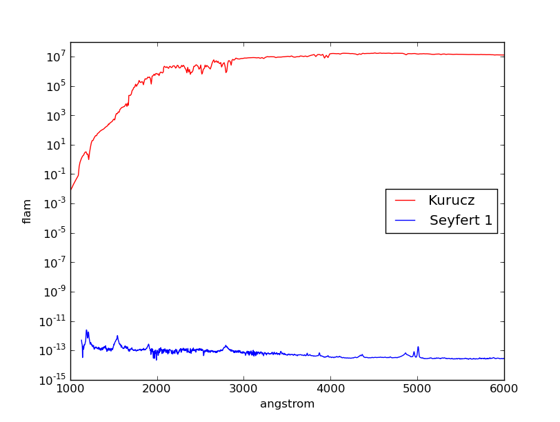
For completeness, the Kurucz spectrum is plotted below in comparison with the Seyfert 1 from above. Note that the Kurucz spectrum has arbitrary flux values and would need to be renormalized (not done here):

>>> plt.semilogy(sp.wave, sp.flux, 'r', label='Kurucz')
>>> plt.semilogy(seyfert1.wave, seyfert1.flux, 'b', label='Seyfert 1')
>>> plt.xlim(1000, 6000)
>>> plt.xlabel(sp.waveunits)
>>> plt.ylabel(sp.fluxunits)
>>> plt.legend(loc='center right')

From File

A source spectrum can also be defined using a FITS or ASCII table containing columns of wavelength and flux. See File I/O for details on how to create such tables.

The example below loads a source spectrum from FITS table, which happens to be one of the HST Calibration Spectra:

>>> filename = os.path.join(
...     os.environ['PYSYN_CDBS'], 'calspec', 'g191b2b_mod_010.fits')
>>> sp = S.FileSpectrum(filename)
>>> sp.flux
array([  6.83127903e-12,   6.83185409e-12,   6.83168973e-12, ...,
         3.47564168e-21,   3.47547205e-21,   3.47530241e-21])

See Tutorial 10 for example on how to load a source spectrum from an ASCII table of any format.

From Arrays

To create a source spectrum from arrays, use ArraySourceSpectrum (also callable as pysynphot.ArraySpectrum). Note in the example below that the flux value of -2 is automatically set to 0, which can be disabled by indicating keepneg=True during initialization:

>>> w = np.array([1000, 2000, 3000])  # Angstrom
>>> f = np.array([1, -2, 3])  # photlam
>>> sp = S.ArraySpectrum(w, f, name='MySource')
Warning, 1 of 3 bins contained negative fluxes; they have been set to zero.
>>> sp.flux
array([ 1.,  0.,  3.])
>>> sp.sample(2500)
1.5

Thermal

ThermalSpectralElement handles a spectral element with thermal properties. It is used in Observation Mode for an IR detector, particularly for thermback() calculation.

For instance, HST/WFC3 IR detector stores thermal information in its $PYSYN_CDBS/comp/wfc3/*_th.fits files. In the table header (extension 1) of each file, there are two keywords:

• DEFT, the detector effective temperature in Kelvin; stored as temperature class attribute

• BEAMFILL, the beam filling factor, usually 1; stored as beamFillFactor class attribute

pysynphot uses this information, applying the thermal emissivity to the optical beam to create a thermal source spectrum, all done behind the scene via ThermalSpectrum(), as follow:

1. Blackbody source spectrum is generated using the DEFT value and the bb_photlam_arcsec() function to calculate flux in photlam per square arcsec.

2. Thermal source spectrum is generated by multiplying the blackbody with ThermalSpectralElement emissivity and BEAMFILL value.

3. If the observation mode has multiple thermal components, their respective thermal source spectra are added together.

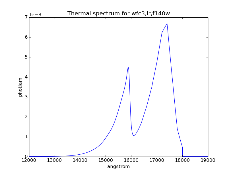
The example below calculates the thermal background (in counts/pixel) for HST/WFC3 IR F140W bandpass and plots its thermal source spectrum:

>>> bp = S.ObsBandpass('wfc3,ir,f140w')
>>> bp.thermback()
0.069428780630446163
>>> thsp = bp.obsmode.ThermalSpectrum()
>>> plt.plot(thsp.wave, thsp.flux)
>>> plt.xlim(12000, 19000)
>>> plt.xlabel(thsp.waveunits)
>>> plt.ylabel(thsp.fluxunits)
>>> plt.title('Thermal spectrum for {0}'.format(bp.obsmode))

Manipulating Source Spectrum

Once you have created a source spectrum, you can manipulate it in several different ways, namely creating a Composite Spectrum from different source spectra and/or bandpass, or applying Extinction, Redshift, or Renormalization.

Composite Spectrum

A composite spectrum is the resultant spectrum from adding, subtracting, or multiplying two spectra, which can be a source spectrum or bandpass. It retains the information of the input spectra as component1 and component2 class attributes. It does not compute the flux or throughput until when explicitly sampled. CompositeSpectralElement handles operations between two bandpasses or between a bandpass and a number, while CompositeSourceSpectrum handles everything else. When an operation involves more than two spectra, the resultant composite spectrum contains other composite spectra from intermediate steps (like a binary tree).

The following table summarizes available operations in pysynphot:

Operand 1	Operation	Operand 2	Result	Commutative
Source Spectrum	\(-\)	Source Spectrum	Composite Source Spectrum	No
Source Spectrum	\(+\)	Source Spectrum	Composite Source Spectrum	Yes
Source Spectrum	\(\times\)	Bandpass	Composite Source Spectrum	Yes
Source Spectrum	\(\times\)	Scalar number	Composite Source Spectrum	Yes
Bandpass	\(\times\)	Bandpass	Composite Spectral Element	Yes
Bandpass	\(\times\)	Scalar number	Composite Spectral Element	Yes

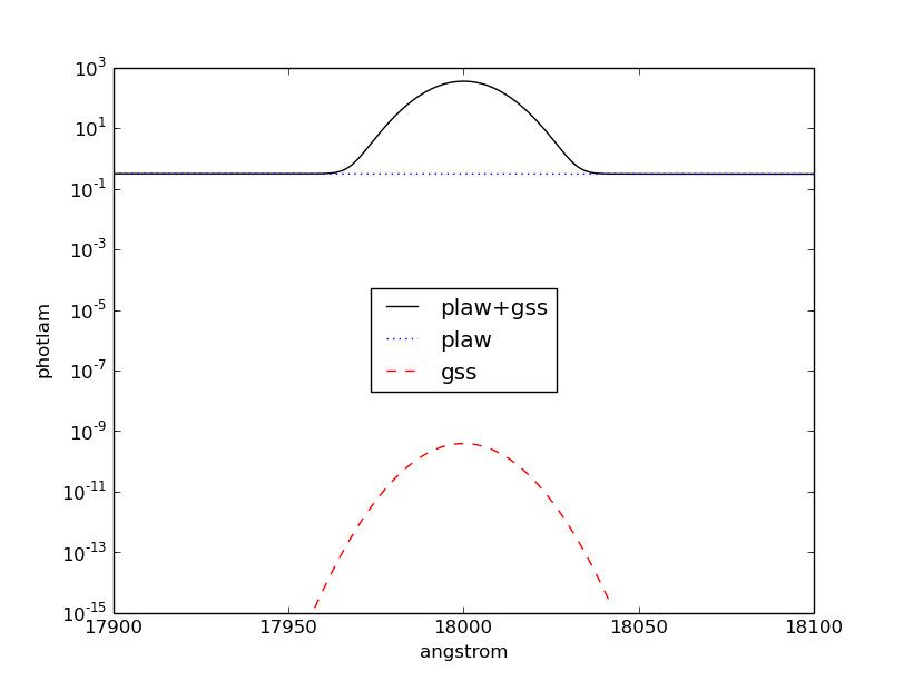
The example below creates a Power-Law source with reference wavelength of 10000 Angstroms and index of -2, and a Gaussian Emission with total flux of \(8.3 \times 10^{-9}\) flam under the curve, central wavelength of 18000 Angstroms, and FWHM of 20 Angstroms. Then, the two spectra are added together to create a new composite source spectrum. They are also all plotted for visualization:

>>> plaw = S.PowerLaw(10000, -2)
>>> gss = S.GaussianSource(8.3e-9, 18000, 20, fluxunits='flam')
>>> sp = plaw + gss
>>> plt.semilogy(sp.wave, sp.flux, 'k', label='plaw+gss')
>>> plt.semilogy(plaw.wave, plaw.flux, 'b:', label='plaw')
>>> plt.semilogy(gss.wave, gss.flux, 'r--', label='gss')
>>> plt.xlim(17900, 18100)
>>> plt.xlabel(sp.waveunits)
>>> plt.ylabel(sp.fluxunits)
>>> plt.legend(loc='center')

Extinction

You can also apply or remove the effects of interstellar reddening on a source spectrum using Extinction by providing a model name and the value of \(E(B-V)\) (negative value effectively de-reddens the spectrum). The extinction is defined as:

\[R(V) = \frac{A(V)}{E(B-V)}\]

Extinction curves for pysynphot has been modeled for different representative regions (see table below). They are available via CRDS (see Installation and Setup) and must be installed under the $PYSYN_CDBS/extinction directory. These are the same models used by Exposure Time Calculator (ETC).

Pre-defined extinction models are as tabulated below. The default model can be specified in three different ways, which are all equivalent. Deprecated models, which are superseded by newer ones but are retained for backward compatibility, are taken from IRAF STSDAS SYNPHOT. The deprecated model, gal2, is not available in pysynphot and will raise an exception if used.

Name	Description	Reference
gal3 mwavg None	Milky Way Diffuse, R(V)=3.1 (Default)	Cardelli et al. (1989)
mwdense	Milky Way Dense, R(V)=5.0
mwrv21	Milky Way CCM, R(V)=2.1
mwrv4	Milky Way CCM, R(V)=4.0
lmc30dor	LMC Supershell, R(V)=2.76	Gordon et al. (2003)
lmcavg	LMC Average, R(V)=3.41
smcbar	SMC Bar, R(V)=2.74
xgalsb	Starburst, R(V)=4.0 (attenuation law)	Calzetti et al. (2000)
gal1	Milky Way (Deprecated)	Seaton (1979)
gal2	Milky Way (Unavailable)	Savage & Mathis (1979)
smc	SMC (Deprecated)	Prevot et al. (1984)
lmc	LMC (Deprecated)	Howarth (1983)
xgal	Extra-galactic (Deprecated)	Calzetti et al. (1994)

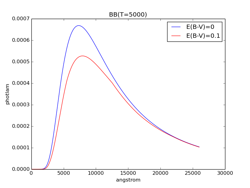
The example below applies LMC (average) extinction with \(E(B-V) = 0.1\) to a blackbody with temperature of 5000 K. Both the original and reddened spectra are plotted for comparison:

>>> sp = S.BlackBody(5000)
>>> sp_ext = sp * S.Extinction(0.1, 'lmcavg')
>>> plt.plot(sp.wave, sp.flux, 'b', label='E(B-V)=0')
>>> plt.plot(sp_ext.wave, sp_ext.flux, 'r', label='E(B-V)=0.1')
>>> plt.xlabel(sp.waveunits)
>>> plt.ylabel(sp.fluxunits)
>>> plt.title(sp.name)
>>> plt.legend(loc='best')

Redshift

In pysynphot, redshifting a source spectrum is done by shifting the flux location by:

\[\lambda_{obs} = (1 + z) \; \lambda_{rest}\]

The flux values themselves are not modified. This functionality is available through the redshift() method, where you provide the value of \(z\). You can also use this method to perform blueshift (see Tutorial 8).

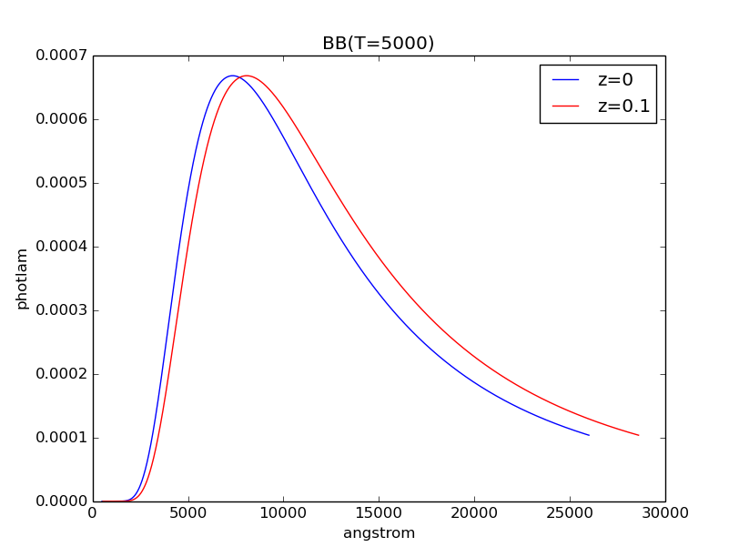
The example below applies \(z = 0.1\) to a blackbody with temperature of 5000 K. Both the original and the redshifted spectra are plotted for comparison:

>>> sp = S.BlackBody(5000)
>>> sp_z = sp.redshift(0.1)
>>> plt.plot(sp.wave, sp.flux, 'b', label='z=0')
>>> plt.plot(sp_z.wave, sp_z.flux, 'r', label='z=0.1')
>>> plt.xlabel(sp.waveunits)
>>> plt.ylabel(sp.fluxunits)
>>> plt.title(sp.name)
>>> plt.legend(loc='best')

Renormalization

A source spectrum can also be renormalized using renorm() to a given flux value and unit in a given bandpass. This is particularly useful when the flux of a source spectrum (e.g., some models in Appendix A: Catalogs and Spectral Atlases) has been arbitrarily renormalized before.

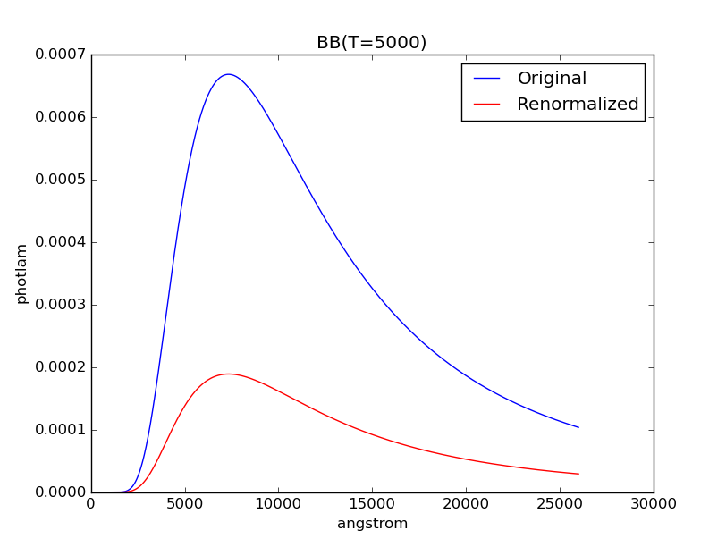
The example below renormalizes a blackbody with temperature of 5000 K to 17 vegamag in Johnson V. Both the original and the renormalized spectra are plotted for comparison:

>>> sp = S.BlackBody(5000)
>>> sp_norm = sp.renorm(17, 'vegamag', S.ObsBandpass('johnson,v'))
>>> plt.plot(sp.wave, sp.flux, 'b', label='Original')
>>> plt.plot(sp_norm.wave, sp_norm.flux, 'r', label='Renormalized')
>>> plt.xlabel(sp.waveunits)
>>> plt.ylabel(sp.fluxunits)
>>> plt.title(sp.name)
>>> plt.legend(loc='best')