Bandpass
A bandpass can be constructed by one of the following methods:
- Specifying a valid string of HST instrument mode keywords (Observation Mode)
- Using a pre-defined function (Box)
- Loading from a FITS or ASCII table
- Using your own wavelength and throughput arrays
It has various photometric properties and these main components:
name(Description of the bandpass; Also accessible via__str__())throughputwave(a.k.a.waveset)waveunits(see Wavelength Units)
To evaluate its transmission at a given wavelength, use its
sample() or
__call__() method, as given in the following example.
Internally, evaluation uses numpy.interp().
>>> bp = S.ObsBandpass('acs,wfc1,f555w')
>>> bp.sample(5000)
0.34331630723608403
>>> bp(5000)
0.34331630723608403
Observation Mode
The observation mode (obsmode) parameter defines the passband, i.e., the
wavelength-dependent sensitivity curve of the photometer or
spectrophotometer. It is controlled by Reference Data.
It can also be used to specify
color index.
The obsmode is usually given as a string of keyword arguments
to the ObsBandpass class.
The list of keywords identify the light path through the telescope and the
instrument, or through a non-HST filter system.
For example, "wfc3,uvis1,f555w" creates a bandpass that is calculated by
taking the product of the individual throughputs of the Wide Field
Camera 3 (WFC3) UVIS Channel 1, the F555W filter, the detector
sensitivity, and the HST Optical Telescope Assembly (OTA). There are special
considerations for OTA and COSTAR.
Another example, "johnson,v" creates a Johnson V bandpass that does not
account for HST optics. A complete list of obsmode keywords can be found in
Appendix B.
Quick Example
Create a bandpass for HST/ACS instrument with its WFC1 detector and F555W filter:
>>> bp_acs = S.ObsBandpass('acs,wfc1,f555w')
To see which throughput tables are being used, as set by Reference Data:
>>> bp_acs.showfiles()
/my/local/dir/trds/comp/ota/hst_ota_007_syn.fits
/my/local/dir/trds/comp/acs/acs_wfc_im123_004_syn.fits
/my/local/dir/trds/comp/acs/acs_f555w_wfc_005_syn.fits
/my/local/dir/trds/comp/acs/acs_wfc_ebe_win12f_005_syn.fits
/my/local/dir/trds/comp/acs/acs_wfc_ccd1_mjd_021_syn.fits
Create a bandpass for Johnson V:
>>> bp_v = S.ObsBandpass('johnson,v')
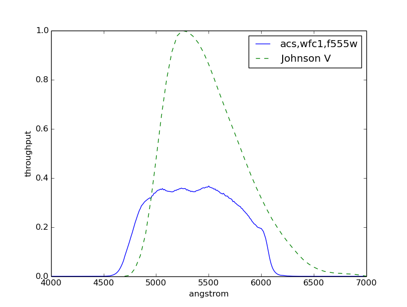
Compare them in a plot:
>>> plt.plot(bp_acs.binset, bp_acs(bp_acs.binset), 'b',
...          bp_v.wave, bp_v.throughput, 'g--')
>>> plt.xlim(4000, 7000)
>>> plt.xlabel(bp_acs.waveunits)
>>> plt.ylabel('throughput')
>>> plt.legend([bp_acs.name, 'Johnson V'], loc='best')
Pixel and Wavelength Ranges
The pixel_range() and
wave_range() methods can be used to
calculate the pixel and wavelength ranges, respectively, spanned by the
observation mode given its binset, if available. For example:
>>> bp = S.ObsBandpass('wfc3,ir,f105w')
To calculate the number of pixels covered from 8600.5 to 12400.5 Angstroms:
>>> bp.pixel_range([8600.5, 12400.5])
3800
To calculate starting and ending wavelengths in Angstroms covered by 3800 pixels centered at 10500 Angstroms:
>>> bp.wave_range(10500.0, 3800)
(8600.5, 12400.5)
Thermal Background
For IR detectors (e.g., NICMOS and WFC3), thermal background can be calculated
using the thermback() method.
The thermal component is defined by thermtable in Reference Data.
For non-IR detectors, calling this method would raise NotImplementedError.
For example:
>>> bp = S.ObsBandpass('wfc3,ir,f105w')
>>> bp.thermback()
0.050852529496148512
>>> bp = S.ObsBandpass('acs,wfc1,f555w')
>>> bp.thermback()
NotImplementedError: No thermal support provided for acs,wfc1,f555w
Box
A box-shaped bandpass is a rectangular window centered on a given wavelength with a given width, both in Angstroms. It is defined as:
where
- \(x_{0}\) is the central wavelength
- \(x\) is the wavelength array
- \(w\) is the width of the box
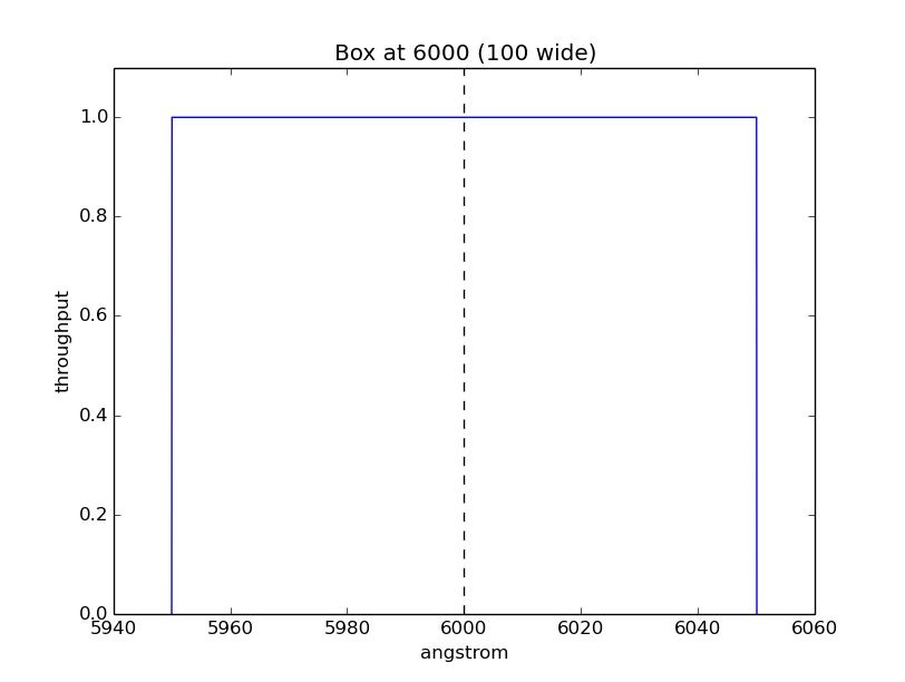
The example below creates and plots a box-shaped bandpass centered at 6000 Angstroms with a width of 100 Angstroms:
>>> bp = S.Box(6000, 100)
>>> plt.plot(bp.wave, bp.throughput)
>>> plt.ylim(0, 1.1)
>>> plt.axvline(6000, ls='--', color='k')
>>> plt.xlabel(bp.waveunits)
>>> plt.ylabel('throughput')
>>> plt.title(bp.name)
Flat
UniformTransmission generates a uniform (flat) bandpass
that has a constant throughput at any wavelength value.
The example below creates and samples a bandpass with a uniform transmission value of 0.8:
>>> bp = S.UniformTransmission(0.8)
>>> bp.sample(5000)
0.8
>>> bp.sample(np.arange(1000, 10000))
array([ 0.8,  0.8,  0.8, ...,  0.8,  0.8,  0.8])
From File
A bandpass can also be defined using a FITS or ASCII table containing columns of wavelength and throughput. See File I/O for details on how to create such tables.
The example below loads a bandpass from FITS table:
>>> filename = os.path.join(
...     os.environ['PYSYN_CDBS'], 'comp', 'acs', 'acs_wfc_ccd2_019_syn.fits')
>>> bp = S.FileBandpass(filename)
>>> bp.throughput
array([  0.00000000e+00,   0.00000000e+00,   1.87380003e-27, ...,
         4.14354995e-09,   0.00000000e+00,   0.00000000e+00])
>>> bp.sample(5100)
0.80144459009170532
>>> bp.sample(2100)
0.0
Tutorial 10: Spectrum from Custom Text File offers hints on how to load a bandpass from an ASCII table of any format.
From Arrays
To create a bandpass from arrays, use ArraySpectralElement
(also callable as pysynphot.ArrayBandpass). Note in the example below that
the bandpass is explicitly tapered at both ends to avoid extrapolation;
Also, unlike source spectrum, its negative throughput value is not automatically
set to zero:
>>> w = np.array([999, 1000, 2000, 3000, 3001])  # Angstroms
>>> t = np.array([0, 0.1, -0.2, 0.3, 0])
>>> bp = S.ArrayBandpass(w, t, name='MyBandpass')
>>> bp.throughput
array([ 0. ,  0.1, -0.2,  0.3,  0. ])
>>> bp.sample(2500)
0.049999999999999989
>>> bp.sample(4000)
0.0
Overlap Checks
To check whether the wavelength range of other bandpass or spectra is defined
everywhere within the main bandpass, you can use the
check_overlap() method, which returns
"full", "partial", or "none". The example below checks whether
the main bandpass overlap with another bandpass of the same detector but with a
different filter, and with a box-shaped one:
>>> bp = S.ObsBandpass('wfc3,ir,f105w')
>>> other_bp = S.ObsBandpass('wfc3,ir,f110w')
>>> bp.check_overlap(other_bp)
'full'
>>> box_bp = S.Box(10000, 10000)
>>> bp.check_overlap(box_bp)
'partial'
To check if the lack of overlap is insignificant, you can use the
check_sig() method. The example
below shows that the partial overlap above is not a concern:
>>> bp.check_sig(box_bp)
True