Appendix C: TMG, TMC, and TMT Files
pysynphot computes the combined throughput for an
observing mode (obsmode) with the
following steps:
- The comma-separated
obsmodeis broken into individual keywords, each becoming a component of theobsmode. - The individual components or keywords are used to search the
graph table, which has 6 columns, starting at the
row with the lowest
INNODEvalue. All rows with thisINNODEare examined. The row whose keyword matches one of the keywords in theobsmodeis selected. If no such row is found, the row with the keyword “default” is selected. If there is no such row and there is only one entry with the currentINNODE, then this row is selected. Otherwise, an exception is raised. - Once the row is selected, the component name that is not “clear” is saved for its throughput lookup in a later step. “Clear” components are discarded because their throughput will not modify the combined throughput.
- The
OUTNODEof the selected row becomes the newINNODE, and the process of searching the graph continues until theOUTNODEis not found in the graph table. For example, see Figure 1. - Once all of the component names are found in the instrument graph
table, the component lookup table
(i.e., the TMC table), which has 4 columns, is searched for the
actual names of the throughput tables, matching by the
COMPNAMEcolumn. For example, see Figure 2. - Once the throughput values are read from the component throughput tables, they are resampled onto the specified wavelength set (if necessary) and multiplied together to form the combined throughput.
The thermback() method actually
traverses the graph table twice; Once in the usual fashion, using the
COMPNAME column; And once to obtain the optical train necessary for thermal
calculations for IR detectors, using the THCOMPNAME column. These trains
differ because of the existence of opaque but emissive components in the optical
path, such as the spider that supports the HST secondary mirror.
The graph table is used to obtain the train of thermally emissive components in the same way it is used for optical components, except that:
obsmodekeywords are compared to the thermal component name (THCOMPNAME) instead of the usualCOMPNAME.- Once all of the component names are found in the graph table, the thermal component lookup table (i.e., the TMT table) is searched for the actual filenames of the emissivity tables. This file has the same format as the TMC file.
Further details and examples can be found in Diaz (2012).
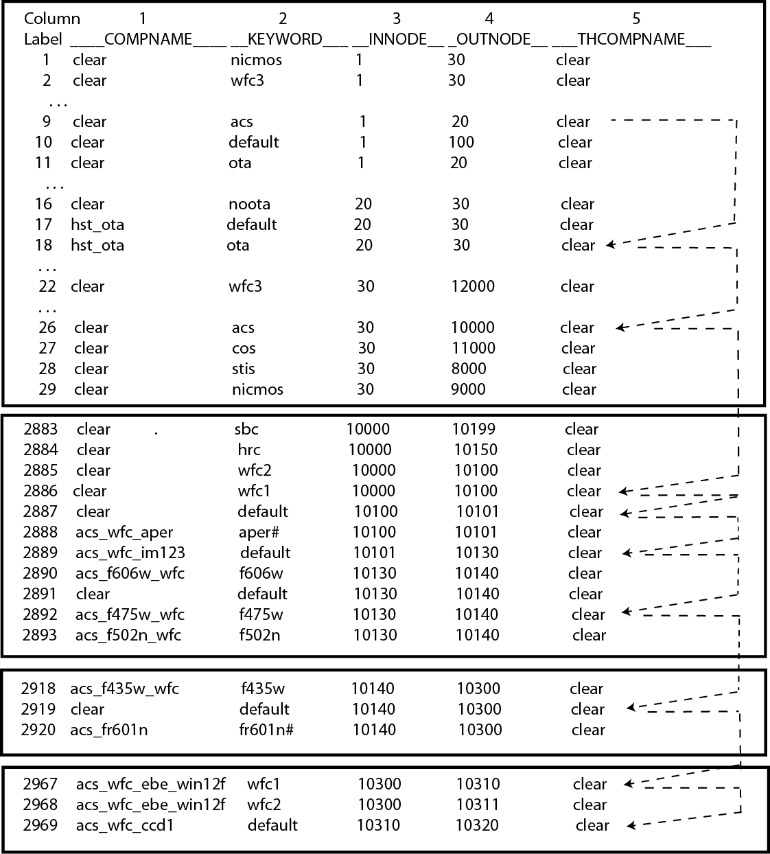
This figure shows the path followed in the graph table (TMG) to gather the components that make the “acs,wfc2,f435w” observing mode. In this example, the keywords are mapped to the components “hst_ota”, “acs_wfc_im123”, “acs_f435w_wfc”, “acs_wfc_ebe_win12f”, and “acs_wfc_ccd1”.
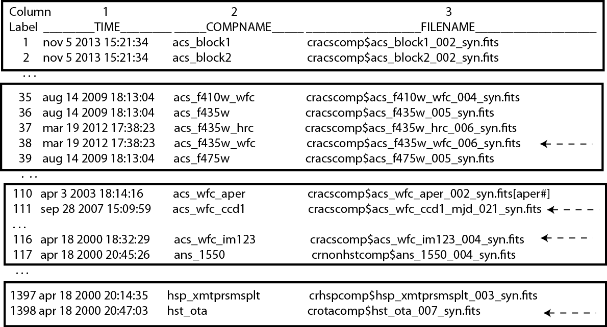
This figure shows the component table (TMC) with the filenames of the components mentioned in Figure 1.
Graph Table (TMG)
The instrument graph table has 6 columns, as follow:
| Column Name | Description | Data Format |
|---|---|---|
| COMPNAME | Component name | String of 20 characters |
| KEYWORD | obsmode keyword |
String of 12 characters |
| INNODE | Input node | Integer |
| OUTNODE | Output node | Integer |
| THCOMPNAME | Thermal component name | String of 20 characters |
| COMMENT [1] | Comment (not used) | String of 68 characters |
| [1] | (1, 2) The comment column is not used by pysynphot. It exists solely for documentation. |
The COMPNAME column contains the name of the component. Each component
must have a unique name, as it is used as primary key for
Component Table (TMC, TMT) lookup. The THCOMPNAME column is similar to
COMPNAME but for Thermal Emissivity Table.
The KEYWORD column is used to match the component keywords in the
obsmode string (also see Appendix B: OBSMODE Keywords). The same component
could be represented by multiple keywords; In that case, it will have multiple
row entries, all of which are identical except for the keywords, in the graph
table. The keyword values are not case-sensitive. The entry for a
parameterized keyword should contain the
keyword followed by a “#” at the end; For example, MJD# and aper# in
Figure 3.
The INNODE and OUTNODE columns specify the light path through the HST.
They are used in the process of searching the graph, as explained
above. Node numbers in those columns should
increase as one goes down the light path in the instrument.
Column         1               2           3          4               5
Label  _____COMPNAME_____ __KEYWORD___ __INNODE__ _OUTNODE__ _____THCOMPNAME_____
1791   clear              default      8224       8225       clear
1792   stis_os21          default      8225       8230       clear
1793   stis_ng21_mjd      MJD#         8230       8233       clear
1794   stis_ng21          default      8230       8233       clear
. . . .
2887   clear              default      10100      10101      clear
2888   acs_wfc_aper       aper#        10100      10101      clear
2889   acs_wfc_im123      default      10101      10130      clear
. . . .
3481   clear              g141         12750      12752      clear
3482   wfc3_ir_g102_bkg   bkg          12701      12800      wfc3_ir_g102_bkg
3483   wfc3_ir_g102_src   default      12701      12800      wfc3_ir_g102_src
3484   wfc3_ir_g102_bkg   bkg          12751      12800      wfc3_ir_g102_bkg
Component Table (TMC, TMT)
TMC and TMT files are the master component and thermal component lookup tables, respectively. Both of them have the same 4 columns, as follow:
| Column Name | Description | Data Format |
|---|---|---|
| TIME [2] | Insertion time (not used) | String of 26 characters |
| COMPNAME | Component name | String of 18 characters |
| FILENAME | Throughput file name and column | String of 50 characters |
| COMMENT [1] | Comment (not used) | String of 68 characters |
| [2] | The insertion time column is used by the pysynphot.
It contains the time that the component file was delivered.
It is included for documentation and to simplify traceability of the
data files. The time format is yyyymmdd:HHMMSS. |
The COMPNAME column is used in TMC and TMT files to link from the
Graph Table (TMG) using the latter’s COMPNAME and THCOMPNAME
columns, respectively.
The FILENAME column provides the filename of the
throughput table, which includes abbreviated
path names, as defined in pysynphot.locations.CONVERTDICT.
The table must be in binary FITS format.
The entry for a parameterized component
should contain its filename followed by square brackets containing the
parameterized keyword; For example,
cracscomp$acs_cor_aper_002_syn.fits[aper#] in Figure 4.
For thermal component, the throughput file should contain
thermal emissivity information
(see Figure 5).
The filenames are not stored directly in the graph table because the files themselves change more frequently than instrument light paths. Therefore, by doing this, we can avoid modifying the more complicated graph table every time a new version of a component throughput is delivered to CRDS.
Column            1                 2                          3
Label _______TIME_________ ___COMPNAME____ ___________________FILENAME__________________ ____________________________COMMENT_____________________________
7    oct 30 2013 15:44:42  acs_blocking3   cracscomp$acs_blocking3_001_syn.fits          throughput curve (all zeroes) for blocking3 filter
8    oct 30 2013 15:44:42  acs_blocking4   cracscomp$acs_blocking4_001_syn.fits          throughput curve (all zeroes) for blocking3 filter
9    apr 03 2003 18:14:16  acs_cor_aper    cracscomp$acs_cor_aper_002_syn.fits[aper#]    acs coronagraph encircled energy table
1   aug 14 2009 18:13:04  acs_f115lp       cracscomp$acs_f115lp_005_syn.fits             updated files. setting throughput zero at end of curves
11   aug 14 2009 18:13:04  acs_f115lp_sbc  cracscomp$acs_f115lp_sbc_004_syn.fits         updated files. setting throughput zero at end of curves
. . . . .
2313 oct 01 2013 19:55:56  stis_ng22       crstiscomp$stis_ng22_016_syn.fits             default date 57113 & end date 57480. turned mjd extrapolation on
2314 oct 01 2013 19:55:56  stis_ng22_mjd   crstiscomp$stis_ng22_mjd_016_syn.fits[mjd#]   default date 57113 & end date 57480. turned mjd extrapolation on
2315 oct 01 2013 19:55:56  stis_ng22b      crstiscomp$stis_ng22b_010_syn.fits            default date 57113 & end date 57480. turned mjd extrapolation on
2316 oct 01 2013 19:55:56  stis_ng22b_mjd  crstiscomp$stis_ng22b_mjd_010_syn.fits[mjd#]  default date 57113 & end date 57480. turned mjd extrapolation on
2317 oct 01 2013 19:55:56  stis_ng23       crstiscomp$stis_ng23_011_syn.fits             default date 57113 & end date 57480. turned mjd extrapolation on
2318 oct 01 2013 19:55:56  stis_ng23_mjd   crstiscomp$stis_ng23_mjd_011_syn.fits[mjd#]   default date 57113 & end date 57480. turned mjd extrapolation on
2319 oct 01 2013 19:55:56  stis_ng24       crstiscomp$stis_ng24_011_syn.fits             default date 57113 & end date 57480. turned mjd extrapolation on
2320 oct 01 2013 19:55:56  stis_ng24_mjd   crstiscomp$stis_ng24_mjd_011_syn.fits[mjd#]   default date 57113 & end date 57480. turned mjd extrapolation on
2321 oct 01 2013 19:55:56  stis_ng31       crstiscomp$stis_ng31_011_syn.fits             default date 57113 & end date 57480. turned mjd extrapolation on
Column            1                 2                          3                                                4
Label __________TIME____________ ___COMPNAME____ __________________FILENAME_________________ __________________COMMENT___________________
 116  aug 15 2006 8:00:00:000am  wfc3_ir_fold    crwfc3comp$wfc3_ir_fold_001_th.fits         Reflectivity of IR fold mirror
 117  aug 15 2006 8:00:00:000am  wfc3_ir_mir1    crwfc3comp$wfc3_ir_mir1_001_th.fits         Reflectivity of IR mirror 1
 118  aug 15 2006 8:00:00:000am  wfc3_ir_mir2    crwfc3comp$wfc3_ir_mir2_001_th.fits         Reflectivity of IR mirror 2
 119  aug 15 2006 8:00:00:000am  wfc3_ir_rcp     crwfc3comp$wfc3_ir_rcp_001_th.fits          Transmission of refractive corrector plate
 120  aug 15 2006 8:00:00:000am  wfc3_ir_wmring  crwfc3comp$wfc3_ir_wmring_001_th.fits       WFC3 warm ring
Throughput Table
The throughput table contains the component throughput as a function of wavelength (see File I/O). It may also contain an optional column of estimated errors or uncertainties associated with the throughput values; The error column must have the following naming convention:
| Wavelength Column Name | Throughput Column Name | Error Column Name |
|---|---|---|
| WAVELENGTH | THROUGHPUT | ERROR |
| <other> (Example: DN1) | <other>_ERR (Example: DN1_ERR) | |
| <other>#<value> (Example: APER#0.1) | <other>_ERR#<value> (Example: APER_ERR#0.1) |
Wavelength values must be in monotonically ascending or descending order. Wavelength unit must be specified for the column (see Wavelength Units for acceptable units). Throughput and error columns do not need units, but you may specify them as “transmission”, “qe”, “dn”, or “photon” (or any of their unique abbreviations) for documentation. Values in all columns must be 64-bit floating-point numbers. Figure 6 shows an example of a simple throughput table.
A component throughput may also be parameterized, meaning that
the throughput is a function of some other variable besides
wavelength. In this case, the table has multiple throughput columns, each
named keyword#value. Examples of such tables are shown in
Figure 7, Figure 8, and Figure 9.
For more details, see Parameterized Keyword.
Column     1           2            3
Label  WAVELENGTH _THROUGHPUT_ ___ERROR____
1      1838.9     0.           INDEF
2      1839.0     1.           INDEF
3      1929.0     1.           INDEF
4      1929.1     0.           INDEF
Column     1            2             3             4             5             6
Label  WAVELENGTH FR647M#5366.0 FR647M#5586.8 FR647M#5807.6 FR647M#6028.4 FR647M#6249.2 ...
1      3500.0     0.            0.            0.            0.            0.            ...
2      3500.2     1.00000E-6    1.00000E-6    1.00000E-6    1.00000E-6    1.00000E-6    ...
3      4829.0     1.96935E-4    8.76876E-5    7.62487E-5    7.39577E-5    7.32903E-5    ...
4      4834.0     2.09608E-4    9.15258E-5    7.94214E-5    7.70256E-5    7.63329E-5    ...
Column       1               2               3               4               5               6
Label __WAVELENGTH___ __THROUGHPUT___ _____ERROR_____ __MJD#50586.0__ __MJD#50959.0__ __MJD#51287.0__
1     1099.           0.              0.              0.              0.              0.
2     1100.           0.9446287       0.              1.              1.011037        1.020443
3     1150.           0.9446287       0.              1.              1.011037        1.020443
Column     1          2          3          4          5          6
Label  WAVELENGTH _APER#0.__ _APER#0.1_ _APER#0.2_ _APER#0.3_ _APER#0.4_
1      3500.      0.28       0.67       0.84       0.88       0.89           ...
2      4000.      0.22       0.68       0.85       0.88       0.9            ...
3      5000.      0.21       0.7        0.86       0.9        0.92           ...
4      6000.      0.22       0.69       0.85       0.9        0.92           ...
Thermal Emissivity Table
The thermal emissivity table contains the component emissivity as a function of wavelength. This is only relevant for IR instruments with non-negligible thermal background. It is similar to throughput table, except that it has the following columns:
- WAVELENGTH
- EMISSIVITY
- ERROR (optional)
Unlike the throughput table, the keyword# parameterization syntax is
overridden for use with the thermal emissivity tables. Instead, this syntax
is used to specify a component temperature, overriding the default temperature
present in the DEFT header keyword (see below).
In addition, it must also contain the following keywords in its table (extension 1) header:
BEAMFILLspecifies the fraction of the optical beam filled by this component. This value is usually 1, but it depends on the precise optical layout of the instrument.DEFTspecifies the default temperature (in Kelvin) of the component. This is the temperature that will be used in thermal calculations unless it is overridden in theobsmode.THTYPEspecifies the type of thermal component that is described by this file:- “opaque” component is the type that partially obstructs the beam. It emits radiation, but does not pass it.
- “thru” component is the type that has both throughput and emissivity. This is the case for most optical elements.
- “numeric” component is the type that does not correspond to a physical device in the instrument, but is represented as such for convenience. For instance, the detector quantum efficiency.
- “clear” component is the type that does not contribute to either throughput or emissivity. It is commonly used as a placeholder in the graph table to organize the flow.
THCOMPNAMEandTHMODEare the associated pair of values used when traversing the graph table.THMODEcontains theobsmodekeyword which points to the associatedTHCOMPNAME.
The example below displays the header keywords mentioned above:
>>> from astropy.io import fits
>>> filename = os.path.join(
...     os.environ['PYSYN_CDBS'], 'comp', 'nicmos', 'nic2_f110w_002_th.fits')
>>> with fits.open(filename) as pf:
...     print(pf[1].header)
....
BEAMFILL=                   1. / Fraction of beam filled by this component
DEFT    =                 77.1 / Default temperature in kelvins
THTYPE  = 'THRU    '           / Thermal type (opaque/thru/numeric/clear)
THCMPNAM= 'nic2_f110w'         / Name of thermal component
THMODE  = 'f110w   '           / Keyword in obsmode to specify temperature
....
Parameterized Keyword
Parameterized keywords are used to access
throughput tables for which the throughput is a
function of some other variables in addition to wavelength.
The syntax for a parameterized keyword is keyword#value, where value is a
numeric (integer or float) value for the keyword to take. The hash sign #
indicates to pysynphot that a parameterized keyword is being used.
A parameterized throughput table contains several throughput columns,
each for a specified value of the parameterized component. When an arbitrary
value is given, pysynphot will linearly interpolate the throughput values
between the two closest keyword values; This is done using the
InterpolatedSpectralElement class. If the table’s
primary (extension 0) header contains PARAMS=WAVELENGTH, wavelength shift
will be done before the interpolation.
Extrapolation is only allowed if the table’s primary header contains an
EXTRAP keyword and it is set to True. Otherwise, the default
THROUGHPUT column will be used (if available) or an exception will be
raised.
The parameterized keywords are also defined in both the
TMG and TMC files.
For TMG, the KEYWORD value will be followed by a “#”; For example, in
Figure 3, “MJD#” indicates that the parameterization is
time dependent, while “aper#” indicates there is a variation in the encircled
energy with aperture size. For TMC, the FILENAME value will be followed
by a “[keyword#]”; For example, in Figure 4, the
“cracscomp$acs_cor_aper_002_syn.fits” file is parameterized by aperture size.
The ACS ramp filter is an example of a parameterized component. The throughput of the ramp filter varies as a function of position (wavelength) on the filter. Therefore, its throughput table contains several throughput columns, each evaluated at a different central wavelength. Figure 7 shows part of the throughput table for ACS FR647M ramp filter, where the first throughput column is for 5366 Angstroms, the second for 5586.8 Angstroms, and so forth. In this case, a request for 5400 Angstroms will result in interpolation between the first two columns.
Another example is the STIS time-dependent
change in sensitivity, as illustrated in Figure 8. In this case,
when “mjd#value” is given as part of an obsmode, the parameterized column(s)
will be used and interpolated, as needed. If “mjd#value” is not given, then the
default THROUGHPUT column is used.
Similarly, parameterization of
encircled energy via aperture size is
shown in Figure 9 for ACS/WFC detector. In this case, the
throughput table is only used when “aper#value” is given in the obsmode,
therefore, a default THROUGHPUT column is unnecessary.
All available parameterized keywords are listed in Appendix B: OBSMODE Keywords
as keyword# or keyword#value.