Observation

Observation is a special type of Source Spectrum, where the source is convolved with a Bandpass, both which are stored in its spectrum and bandpass class attributes, respectively.

It also has two different datasets:

• wave and flux, as defined by the native wavelength set, which is constructed when combining the source spectrum and the bandpass.
• binwave and binflux, as defined by the binned wavelength set.

Binned wavelength set uses the optimal binning for the detector, if applicable. When optimal binning is not found (e.g., a non-HST filter system), it uses the native wavelength set instead (see Reference Data). For IRAF STSDAS SYNPHOT users, this is the same behavior as the countrate task. In addition, binwave can be explicitly overwritten using the binset keyword at initialization. Note that the given array must contain the central wavelength values of the bins.

Once binwave is established, binflux is computed by integrating the native flux over the width of each bin. Due to the nature of binned data, binflux cannot be interpolated when sampled. To accurately represent binned dataset in a plot, you should plot it as a histogram, with each binwave value at the mid-point of the horizontal step (see Examples).

In contrast, the native dataset is considered to be samples of a continuous function. Thus, it may be interpolated linearly and plotted without using a histogram.

An observation can be sampled using its sample() method. By default, it samples the binned dataset and does not allow interpolation; i.e., you must provide a wavelength value that exactly match that in binwave. It will sample the native dataset and allows interpolation if the binned=False option is used. For for information, see Sampling.

The following operations are disabled because they do not make sense in the context of an observation, in which a photon has passed through the telescope optics:

• Redshift
• Addition/subtraction
• Some multiplication (see below)

When multiplication is performed, a new observation is created using its original source spectrum and a new bandpass from multiplying its original bandpass with the given bandpass or scalar number. An observation cannot be multiplied with another observation, source spectrum, or extinction curve.

In addition, it has unique properties, such as Effective Stimulus (also see Count Rate) and Effective Wavelength.

Like a source spectrum, an observation can be written to a FITS table using its writefits() method (also see File I/O), which in this case, takes an additional binned keyword to indicate which dataset to write.

Count Rate

countrate() is probably the most often used method for an observation. It computes the total counts of a source spectrum, integrated over the passband defined by a HST observing mode. For calculations, it uses an optimal wavelength set (if available), which is constructed so that one wavelength bin corresponds to one detector pixel.

It has two unique features below that are helpful when simulating a HST observation. Therefore, it is ideally suited for predicting exposure times (e.g., using HST ETC) when writing HST proposals:

1. The input parameters were originally structured to mimic what is contained in the exposure logsheets found in HST observing proposals in Astronomer’s Proposal Tool (APT).
2. For the spectroscopic instruments, it will automatically search for and use a wavelength table that is appropriate for the selected instrumental dispersion mode.

Examples its usage are available in Examples, Tutorial 1: Observation, and Tutorial 7: Count Rates for Multiple Apertures.

Sampling

sample() is another useful method for an observation. It allows the computation of the number of counts at a particular reference wavelength (in Angstroms) for either binned or native dataset.

The example below computes the number of counts for Vega at 10000 Angstroms, as observed by HST/WFC3 IR detector using F105W filter:

>>> refwave = 10000
>>> obs = S.Observation(S.Vega, S.ObsBandpass('wfc3,ir,f105w'))
>>> obs.sample(refwave)  # Binned dataset
6427997.452742151
>>> obs.sample(refwave, binned=False)  # Native dataset
32194062.511316653

In contrast, its __call__() method is the same as Source Spectrum. It always computes flux in photlam and can only “see” the native dataset, as illustrated by the example below:

>>> obs(refwave)
142.0874566775498

Examples

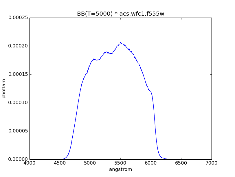
Simulate an observation of a 5000 K blackbody through the HST/ACS WFC1 F555W bandpass, and plot its binned dataset:

>>> obs = S.Observation(S.BlackBody(5000), S.ObsBandpass('acs,wfc1,f555w'))
>>> plt.plot(obs.binwave, obs.binflux, drawstyle='steps-mid')
>>> plt.xlim(4000, 7000)
>>> plt.xlabel(obs.waveunits)
>>> plt.ylabel(obs.fluxunits)
>>> plt.title(obs.name)

Calculate the count rate of this observation in the unit of counts/s over the HST collecting area (i.e., the primary mirror) that is defined in \(\mathrm{cm}^{2}\):

>>> obs.primary_area
45238.93416
>>> obs.countrate()
10080.633086603169

Calculate the effective stimulus in flam:

>>> obs.effstim('flam')
1.9951166916464598e-15

Calculate the effective wavelength in Angstroms:

>>> obs.efflam()
5406.9723492971034

Convert the flux unit to counts:

>>> obs.convert('counts')

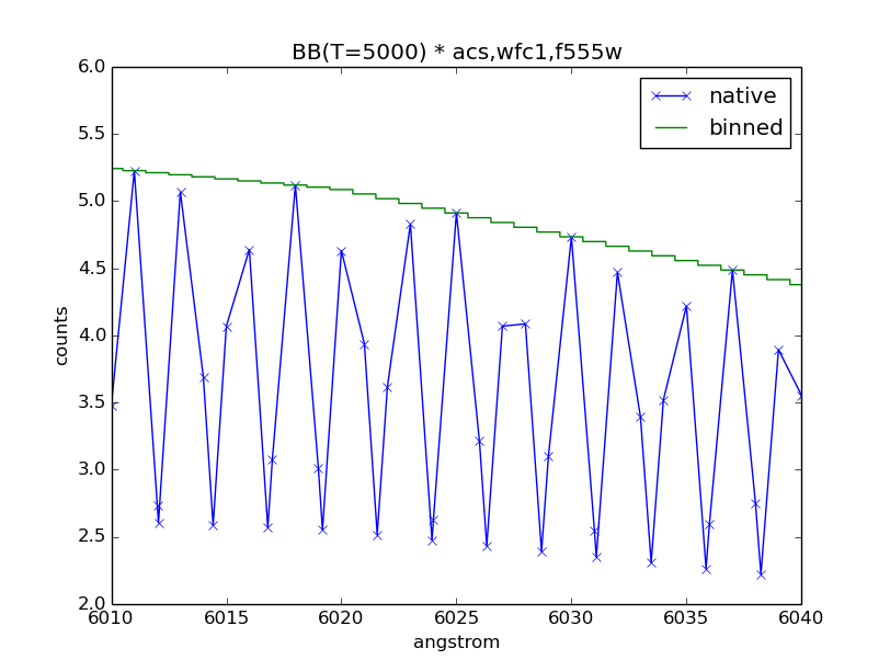
Plot observation data in both native and binned wavelength sets. Note that counts per wavelength bin depends on the size of the bin because it is not a flux density:

>>> plt.plot(obs.wave, obs.flux, marker='x', label='native')
>>> plt.plot(obs.binwave, obs.binflux, drawstyle='steps-mid', label='binned')
>>> plt.xlim(6010, 6040)
>>> plt.ylim(2, 6)
>>> plt.xlabel(obs.waveunits)
>>> plt.ylabel(obs.fluxunits)
>>> plt.title(obs.name)
>>> plt.legend(loc='best')

Write the observation out to two FITS tables, one with native dataset and the other binned:

>>> obs.writefits('myobs_native.fits', binned=False)
>>> obs.writefits('myobs_binned.fits')